The Gradient Boosters VI(A): Natural Gradient

We are taking a brief detour from the series to understand what Natural Gradient is. The next algorithm we examine in the Gradient Boosting world is NGBoost and to understand it completely, we need to understand what Natural Gradients are.

Pre-reads: I would be talking about KL Divergence and if you are unfamiliar with the concept, take a pause and catch-up. I have another article where I give the maths and intuition behind Entropy, Cross Entropy and KL Divergence.
I also assume basic familiarity with Gradient Descent. I’m sure you’ll find a million articles about Gradient Descent online.

Sometimes, during the explanation, we might take on some maths heavy portions. But wherever possible, I’ll also provide the intuition so that if you are averse to maths and equations, you can skip right to the intuition.

Gradient Descent

There are a million articles on the internet explaining what Gradient Descent is and this is not the million and one article. Briefly, we will just cover enough Gradient Descent to make the discussion ahead relevant.

The Problem setup is : Given a function f(x), we want to find its minimum. In machine learning, this f(x) is typically a loss function, and x is the parameters of the algorithm(for eg. in Neural Networks x is the weights and biases of the network).

We pick an initial value for x, mostly at random,
We calculate the gradient of the loss function w.r.t. the parameters x, $\frac{\partial f(x)}{\partial x}$
We adjust the parameters x, such that $x = x - \alpha \frac{\partial f(x)}{\partial x}$ , where $\alpha$ is the learning rate
Repeat 2 and 3 until we are satisfied with the loss value.

For a more mathematical formulation of Gradient Descent you can visit Sebastian Raschka’s mlxtend

There are two main ingredients to the algorithm – the gradient and the learning rate.

Gradient is nothing but the first derivative of the loss function w.r.t. x. This is also called the slope of the function at the point. From high-school geometry, we know that slope can have sign and depending on the sign we know which direction is “down”. For eg. in the picture above, the gradient or slope is negative and we know we have to move in the negative direction to reach the minima. So the gradient also gives you the direction in which you need to move and it is this property that Gradient Descent uses.

Learning Rate is a necessary scaling which is applied to the gradient update every time. It is just a small quantity by which we restrain the parameter update based on the gradient to make sure our algorithm converges. We will discuss why we need this very soon.

Limitations

The first pitfall of Gradient Descent is the step size. We adjust the parameters, x, using the gradient of the loss function(scaled by learning rate).

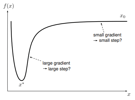
The gradient is the first derivative of the loss function and by definition, it only knows the slope at the point at which it was calculated. It is myopic towards what the slope is even a point at an infinitesimally small distance. In the diagram above, we can see two points, and the one on the steep drop has a higher gradient value and the one on the almost flat has a smaller gradient. But does that mean we should be taking larger or smaller steps respectively? Because of this we can only take the direction the gradient gives us as the absolute truth and manage the step size using a hyperparameter learning rate. This hyperparameter makes sure we do not jump over the minima(if the step size is too high) or never reach the minima (if the step size is too small).

This is a pitfall you can find in almost all first order optimization algorithms. One way to solve it is to use the second derivative which also tells you the curvature of the function and make the update step based on that, which is what Newton Raphson method of optimization does (Appendix in one of the previous blog post). But second order optimization methods come with their own baggage – computational and analytical complexity.

Another pitfall is the fact that this update treats all the parameters the same by scaling everything by a learning rate. There might be some parameters which have a larger influence on the loss function than other and by restricting the update for such parameters, we are making the algorithm longer to converge.

The Alternative

What’s the alternative? The constant learning rate update is like a safety cushion we are giving the algorithm so that it doesn’t blindly dash from one point to the other and miss the minima altogether. But there is another way we can implement this safety cushion.

Instead of fixing the euclidean distance each parameter moves(distance in the parameter space), we can fix the distance in the distribution space of the target output. i.e. Instead of changing all the parameters within an epsilon distance, we constrain the output distribution of the model to be within an epsilon distance from the distribution from the previous step.

Now how do we measure the distance between two distributions? Kullback-Leibler Divergence. Although technically not a distance(because it is not symmetric), it can be considered a distance in the locality it is defined. This works out well for us because we are also concerned about how the output distribution changes when we make small steps in the parameter space. In essence, we are not moving in the Euclidean parameter space like in normal gradient descent. but in the distribution space with KL Divergence as the metric.

Fisher Information Matrix and Natural Gradient

I’ll skip to the end and tell you that there is this magical matrix called the Fischer Information Matrix, which if we include in the regular gradient descent formula, we will get the Natural Gradient descent which has the property of constraining the output distribution in each update step[1].

$x_{t+1} = x_t - \eta_t \cdot F(\theta_t)^{-1} \cdot \frac{\partial f(x)}{\partial x}$

This is exactly the gradient descent equation, with a few changes:

$\alpha$ , the learning rate, is replaced with $\eta_t$ to make it clear that the step size may change in each iteration
An additional term $F(\theta_t)^{-1}$ has been added to the normal gradient.

When the normal gradient is scaled with the inverse of the Fisher’s matrix, we call it the Natural Gradient.

Now for those who can accept the hand-wave that Fisher Matrix is a magical quantity which makes the normal gradient natural, skip to the next section. For the brave souls who stick around, a little maths is on your way.

Math(Fisher Matrix)

I assume everyone knows what KL divergence is. We are going to start with KL Divergence and see how that translates to Fisher Matrix and what is the Fisher Matrix.

As we saw in the Deep Learning and Information Theory, KL Divergence was defined as:

$KL(P||Q) = \sum_{x}p(x) log(\frac{p(x)}{q(x)})$

That was when we were talking about a discrete variable, like a categorical outcome. In a more general sense, we need to replace the summations with integration. Let’s also switch the notation to suit the gradient descent framework that we are working with.

Instead of P and Q as two distributions, let’s say $p(x;\theta)$ and $p(x;\theta+\delta\theta)$ be the two distributions, where x is our input features or covariates, $\theta$ be the parameters of the loss function(for eg. the weights and biases in a neural network), and $\delta\theta$ be the small change in parameters that we make in a gradient update step. So, under the new notation, the KL Divergence is defined as:

$KL(p(x;\theta)||p(x;\theta+\delta\theta)) = \int p(x;\theta) log(\frac{p(x;\theta)}{p(x;\theta+\delta\theta)}) dx$

$=\int p(x;\theta) \cdot log(p(x;\theta))dx - \int p(x;\theta) \cdot log(p(x;\theta+\delta\theta)) dx$

Let’s rewrite the second term of the equation in terms of $p(x;\theta)$ using second-order Taylor Expansion(which is an approximation using the derivatives at a particular point). Taylor Expansion in it’s general form is:

$f(\theta) \approx f(\theta_t) + \triangledown f(\theta_t)^T\cdot\delta\theta + \frac {1}{2}\cdot \delta\theta^T\cdot (\triangledown^2 f(\theta)) \cdot \delta\theta$

Rewriting the second term in this form, we get:

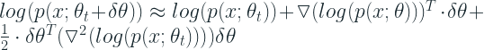
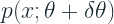
$log(p(x;\theta_t+\delta\theta)) \approx log(p(x;\theta_t)) + \triangledown (log(p(x;\theta)))^T\cdot\delta\theta + \frac {1}{2} \cdot \delta\theta^T (\triangledown^2(log(p(x;\theta_t))))\delta \theta$

Let’s whip out our trusty Chain rule from high school calculus and apply to the first term. Derivative of Log x is 1/x. The Taylor Expansion of the second term becomes:

$log(p(x;\theta_t+\delta\theta)) \approx log(p(x;\theta_t)) + (\frac {\triangledown (p(x;\theta))}{p(x;\theta_t)})^T \cdot\delta\theta + \frac {1}{2} \cdot \delta\theta^T (\triangledown^2(log(p(x;\theta_t))))\delta \theta$

Plugging this back into the KL Divergence equation,. we get:

$\int p(x;\theta_t) \cdot log ;p(x;\theta_t) dx - \int p(x;\theta_t);\cdot (log;p(x;\theta_t)+ (\frac {\triangledown p(x;\theta_t)}{p(x;\theta_t)})^T\cdot \delta\theta + \frac {1}{2}\cdot \delta\theta^T \cdot (\triangledown^2 log;p(x;\theta_t)\delta\theta) dx$

Rearranging the terms we have:

$\int p(x;\theta_t) \cdot \frac {log ;p(x;\theta_t)}{log ;p(x;\theta_t)} dx - (\int \triangledown p(x;\theta_t)dx)^T\cdot\delta\theta - \frac{1}{2} \cdot \delta\theta^T\cdot(\int p(x;\theta_t) \cdot \triangledown^2 log ; p(x;\theta_t)) \cdot \delta \theta$

The first term is the KL Divergence between the same distribution and that is going to be zero. Another way you can think about it is that log 1 = 0 and hence the first term becomes zero.

The second term will also be zero. Let’s take a look at that below. Key property which we use to infer zero is that the integration of a probability distribution P(x) with x is 1 (just like the summation of the area under the curve of a probability distribution is 1).

$\int \triangledown p(x;\theta_t)dx = \triangledown \int p(x;\theta_t)dx = \triangledown 1 = 0$

Now, that leaves us with the Hessian of $log\; p(x;\theta_t)$ . A little bit of mathematics(*hand-wave*) gets us:

$\triangledown^2 log\;p(x;\theta_t) = \frac {1}{p(x;\theta_t)} \cdot \triangledown^2 p(x;\theta_t) - \triangledown log;p(x;\theta_t) \cdot \triangledown log;p(x;\theta_t)^T$

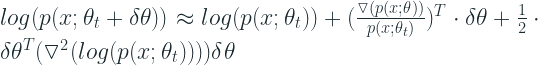
Let’s put this back into the KL Divergence equation.

$KL(p(x;\theta_t) || p(x;\theta_t+\delta\theta)) \approx -\frac {1}{2} \cdot \delta\theta^T \cdot \int \triangledown^2 p(x;\theta_t)dx \cdot \delta\theta + \frac {1}{2}\cdot \delta\theta^T (\int p(x;\theta_t) [\triangledown log; p(x;\theta_t); \triangledown log;p(x;\theta_t)^T]dx) \delta\theta$

The first term becomes zero because as we saw earlier, the integral of a probability distribution P(x) over x is 1. And the first and second derivative of 1 is 0. In the second term, the integral is called the Fisher’s matrix. Let’s call it F. So the KL Divergence equation becomes:

$KL(p(x;\theta_t) || p(x;\theta_t+\delta\theta)) \approx \frac {1}{2} \cdot \delta\theta^T \cdot F \cdot \delta\theta$

Intuition(Fisher Matrix)

The integral over x in the Fisher matrix can be interpreted as the Expected Value. And what that makes the Fisher Matrix is the negative Expected Hessian of $log;p(x;theta_t)$ . And $log;p(x;theta_t)$ is nothing but the log likelihood. We know that the first derivative gives us the slope and the second derivative(Hessian) gives us the curvature. So, the Fisher Matrix can be seen as the curvature of the log likelihood function.

The Fisher Matrix is also the covariance of the score function. In our case the score function is the log likelihood which measures the goodness of our prediction.

Math(Natural Gradient)

We looked at what Fisher Matrix is, but we still haven’t linked it to Gradient Descent. Now, we know that KL Divergence is a function of Fisher Matrix and the delta change in parameters between the two distributions. As we discussed earlier, our aim is to make sure that we minimize the loss subject to keeping the KL Divergence within a constant c.

Formally, it can be written as:

$\delta\theta^* = \underset{\delta\theta ; s.t. KL(p_{\theta}||p_{\theta+\delta\theta})=c}{argmin} L(\theta_t + \delta\theta)$

Let’s take the Lagrangian relaxation of the problem and use our trusted first order Taylor relaxation for the $L(\theta_t + \delta\theta)$

$\delta\theta^* = \underset{\delta\theta}{argmin} ;L(\theta_t + \delta\theta) + \lambda (KL(p_{\theta}||p_{\theta+\delta\theta})-c)$

$\approx \underset{\delta\theta}{argmin} ;(L(\theta_t) + \triangledown L(\theta)^T\delta\theta + \frac {1}{2}\cdot \lambda\cdot\delta\theta^T\cdot F \cdot \delta\theta - \lambda c)$

To minimize the function above, we set the derivative to zero and solve. The derivative of the above function is:

$\triangledown L(\theta_t)) + \lambda F \delta\theta$

Setting it to zero and solving for $\delta\theta$ , we get,

$\delta\theta = -\frac {1}{\lambda} F^{-1} \triangledown L(\theta)$

What this means is that to a factor of $\frac{1}{\lambda}$ (this is the error tolerance we accepted with the Lagrangian Relaxation), we get the optimal descent direction taking into account the curvature of the log likelihood at that point. We can take this constant factor of relaxation into the learning rate and consider it part of the same constant.

And with that final piece of mathematical trickery, we have the Natural Gradient as,

$\tilde {\triangledown}_{\theta} L(\theta) = F^{-1} \triangledown_{\theta} L(\theta)$

Gradient vs Natural Gradient

We’ve talked a lot about Gradients and Natural Gradients. But it is critical to understand why Natural Gradient is different from normal gradient to understand how Natural Gradient Descent is different from Gradient Descent.

At the center of it all, is a Loss Function which measures the difference between the predicted output and the ground truth. And how do we change the loss? By changing the parameters which changes the predicted output and thereby the loss. So, in a normal Gradient, we take the derivative of the loss function w.r.t. the parameters. The derivative will be small if the predicted probability distribution is closer to the true distribution and vice versa This represents the amount your loss would change if you moved each parameter by one unit. So, when we apply the learning rate, we are scaling the gradient update to these parameters by a fixed amount.

In the Natural Gradient world, we are no longer restricting the movement of the parameters in the parameter space. Instead, we arrest the movement of the output probability distribution at each step. And how do we measure the probability distribution? Log Likelihood. And Fisher Matrix gives you the curvature of the Log Likelihood.

As we saw earlier, the normal gradient has no idea about the curvature of the loss function because it is a first order optimization method. But when we include the Fisher matrix to the gradient, what we are doing is scaling the parameter updates with the curvature of the log likelihood function. So, places in the distribution space where the log likelihood changes fast w.r.t. a parameter, the update for the parameter would be less as opposed to a flat plain in the distribution space.

Apart from the obvious benefit of adjusting our updates using the curvature information, Natural Gradient also allows a way for us to directly control the movement of your model in the predicted space. In normal gradient, your movement is strictly in the parameter space and we are restricting the movement in that space with a learning rate in the hope that the movement in the prediction space is also restricted. But in Natural Gradient update, we are directly restricting the movement in the prediction space by stipulating that the model only move a fixed distance in KL Divergence terms.

So.. Why am I hearing about this only now?

The obvious question is a lot of your minds would be: If Natural Gradient Descent is so awesome, and clearly better than Gradient Descent, why isn’t it the defacto standard in Neural Networks?

This is one of those areas where pragmatism won over theory. Theoretically, the idea of using Natural Gradients is beautiful and it works also as expected. But the catch is that the calculation of the Fisher Matrix and it’s inverse becomes an intractable problem when the number of parameters are huge, like in a typical Deep Neural Network. This calculation exists in $n\_parameter^2$ .

One other reason why there wasn’t a lot of focus on Natural Gradients was that the Deep Learning researchers and practitioners figured out some clever tricks/heuristics to approximate the information in a second derivative without calculating it. The Deep Learning optimizers have come a long way from SGD and a lot of that progress has been in using such tricks to get better gradient updates. Momentum, RMSProp, Adam, are all variations of the SGD which uses a running mean and/or running variance of the gradients to approximate the second order derivative and use that information to do the gradient updates.

These heuristics are much less computationally intensive that calculating a second order derivative or the natural gradient and has enabled Deep Learning to be scaled to the level it is currently.

That being said, the Natural Gradient still finds use in some cases where the parameters to be estimated are relatively small, or the expected distribution is relatively standard like a Gaussian distribution, or in some areas of Reinforcement Learning. Recently, it has also been used in a form of Gradient Boosting, which we will cover in the next part of the series.

In the next part of our series, let’s look at the new kid on the block – NgBoost

Part I – Gradient boosting Algorithm
Part II – Regularized Greedy Forest
Part III – XGBoost
Part IV – LightGBM
Part V – CatBoost
Part VI(A) – Natural Gradient
Part VI(B) – NGBoost
Part VII – The Battle of the Boosters

References

Amari, Shun-ichi. Natural Gradient Works Efficiently in Learning. Neural Computation, Volume 10, Issue 2, p.251-276.
It’s Only Natural: An Excessively Deep Dive into Natural Gradient Optimization, https://towardsdatascience.com/its-only-natural-an-excessively-deep-dive-into-natural-gradient-optimization-75d464b89dbb
Ratliff, Nathan ,Information Geometry and Natural Gradients, https://ipvs.informatik.uni-stuttgart.de/mlr/wp-content/uploads/2015/01/mathematics_for_intelligent_systems_lecture12_notes_I.pdf
Natural Gradient Descent, https://wiseodd.github.io/techblog/2018/03/14/natural-gradient/
Fisher Information Matrix, https://wiseodd.github.io/techblog/2018/03/11/fisher-information/
What is the natural gradient, and how does it work?, http://kvfrans.com/what-is-the-natural-gradient-and-where-does-it-appear-in-trust-region-policy-optimization/

5 thoughts on “The Gradient Boosters VI(A): Natural Gradient”

Pingback: The Gradient Boosters VI(B): NGBoost – Deep & Shallow
Pingback: The Gradient Boosters V: CatBoost – Deep & Shallow
Pingback: The Gradient Boosters IV: LightGBM – Deep & Shallow
Pingback: The Gradient Boosters VII: Battle of the Boosters – Deep & Shallow
hello says:

August 31, 2022 at 7:23 pm

thank you for your post, it’s very useful

LikeLike

The Gradient Boosters VI(A): Natural Gradient