

We have come a long way in the world of Gradient Boosting. If you have followed the whole series, you should have a much better understanding about the theory and practical aspects of the major algorithms in this space. After a grim walk through the math and theory behind these algorithms, I thought it would be a fun change to see all of them in action in a highly practical blog post.
So, I present to you, the Battle of the Boosters.
The Datasets
I have chosen a few datasets for regression from Kaggle Datasets, mainly because it’s easy to setup and run in Google Colab. Another reason is that I do not need to spend a lot of time in data preprocessing, instead I can pick one of the public kernels and get cracking. I’ll also share one kernel for EDA of the datasets we choose. All notebooks will also be shared and links at the bottom of the blog.
- AutoMPG – The data is technical spec of cars from UCI Machine Learning Repository.
Shape: (398,9) , EDA Kernel, Data Volume: Low - House Prices: Advanced Regression Techniques – The Ames Housing dataset was compiled by Dean De Cock for use in data science education. It’s an incredible alternative for data scientists looking for a modernized and expanded version of the often cited Boston Housing dataset. With 79 explanatory variables describing (almost) every aspect of residential homes in Ames, Iowa, this competition challenges you to predict the final price of each home.
Shape: (1460, 81), EDA kernel, Data Volume: Medium - Electric Motor Temperature – The data set comprises several sensor data collected from a permanent magnet synchronous motor (PMSM) deployed on a test bench. The PMSM represents a German OEM’s prototype model.
Shape: (998k,13), EDA Kernel, Data Volume: High
Experimental Setup
Algorithms in Contention
- XGBoost
- LightGBM
- Regularized Greedy Forest
- NGBoost
Data Preprocessing
Nothing fancy here. Just did some basic data cleansing and scaling. Most of the code is from some random kernel. The only point is that the same preprocessing is applied to all algorithms
Cross Validation Setup
I have chosen cross validation to make sure the comparison between different algorithms is more generalized than specific to one particular split of the data. I have chosen a simple K-Fold with 5 folds for this exercise.
Evaluation
Evaluation Metric : Mean Squared Error
To have standard evaluation for all the algorithms(thankfully all of them are Sci-kit Learn api), I defined a couple of functions.
Default Parameters: First fit the CV splits with default parameters of the model. We record the mean and standard deviation of the CV scores and then fit the entire train split to predict on the test split.
def eval_algo_sklearn(alg, x_train, y_train,x_test, y_test, cv):
    MSEs=ms.cross_val_score(alg, x_train, y_train, scoring='neg_mean_squared_error', cv=cv)
    meanMSE=np.mean(MSEs)
    stdMSE = np.std(MSEs)
    alg=alg.fit(x_train,y_train)
    pred=alg.predict(x_test)
    rmse_train = math.sqrt(-meanMSE)
    rmse_test = math.sqrt(sklm.mean_squared_error(y_test, pred))
    return rmse_train, stdMSE, rmse_test
With Hyperparameter Tuning: Very similar to the previous one, but with an additional step of GridSearch to find best parameters.
def tune_eval_algo_sklearn(alg, param_grid, x_train, y_train, x_test, y_test, cv):
    grid=GridSearchCV(alg, param_grid=param_grid, cv=cv, scoring='neg_mean_squared_error', n_jobs=-1)
    grid.fit(x_train,y_train)
    print(grid.best_estimator_)
    best_params = grid.best_estimator_.get_params()
    alg= clone(alg).set_params(**best_params)
    alg=alg.fit(x_train,y_train)
    pred=alg.predict(x_test)
    rmse_train = math.sqrt(-grid.cv_results_['mean_test_score'][grid.best_index_])
    stdMSE = grid.cv_results_['std_test_score'][grid.best_index_]
    rmse_test = math.sqrt(sklm.mean_squared_error(y_test, pred))
    return rmse_train, stdMSE, rmse_test, alg
Hyperparameter tuning is in no way exhaustive, but is fairly decent.
The grids over which we run GridSearch for the different algorithms are
XGBoost:
{
    "learning_rate": [0.01, 0.1, 0.5],
    "n_estimators": [100, 250, 500],
    "max_depth": [3, 5, 7],
    "min_child_weight": [1, 3, 5],
    "colsample_bytree": [0.5, 0.7, 1],
}
LightGBM:
{
    "learning_rate": [0.01, 0.1, 0.5],
    "n_estimators": [100, 250, 500],
    "max_depth": [3, 5, 7],
    "min_child_weight": [1, 3, 5],
    "colsample_bytree": [0.5, 0.7, 1],
}
RGF:
{
    "learning_rate": [0.01, 0.1, 0.5],
    "max_leaf": [1000, 2500, 5000],
    "algorithm": ["RGF", "RGF_Opt", "RGF_Sib"],
    "l2": [1.0, 0.1, 0.01],
}
NGBoost:
Because NGBoost is kinda slow, instead of defining a standard grid for all experiments, I have done search along each parameter, independently, and decided a grid based on the intuitions from that experiment
Results
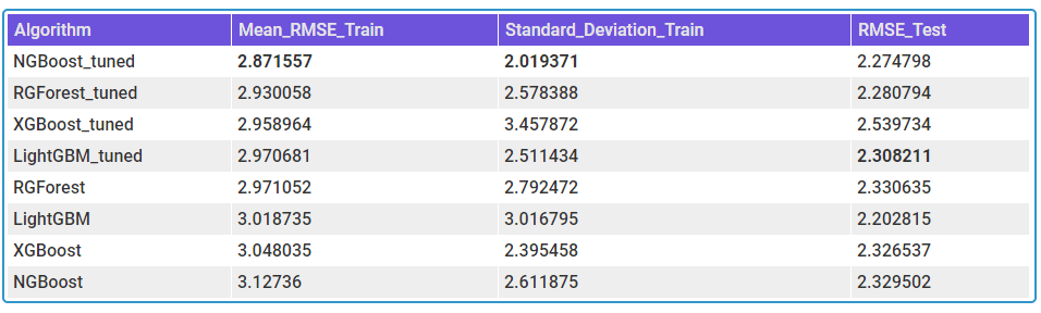
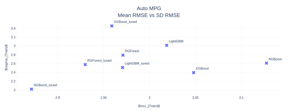
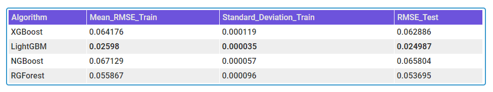
I’ve tabulated the Mean and Standard Deviations of RMSEs for the Train CV splits for all three datasets. For Electric-Motors, I did not tune the data, as it was computationally expensive.
AutoMPG
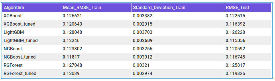
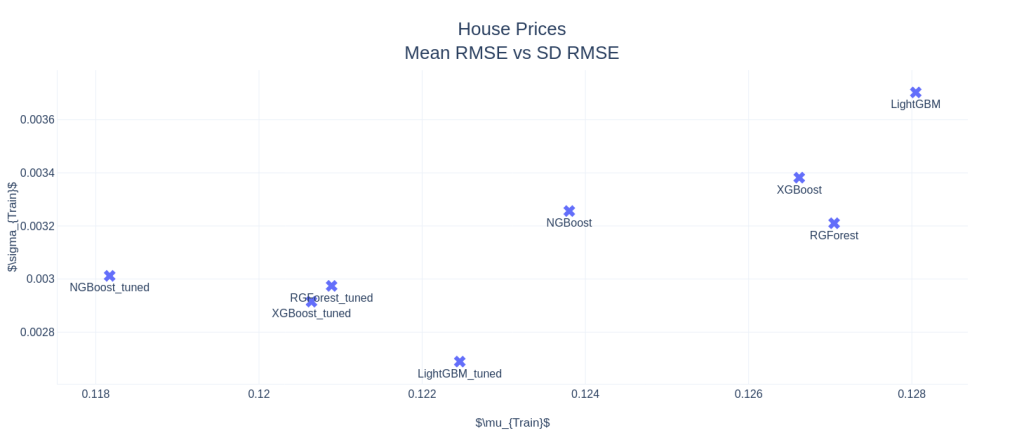
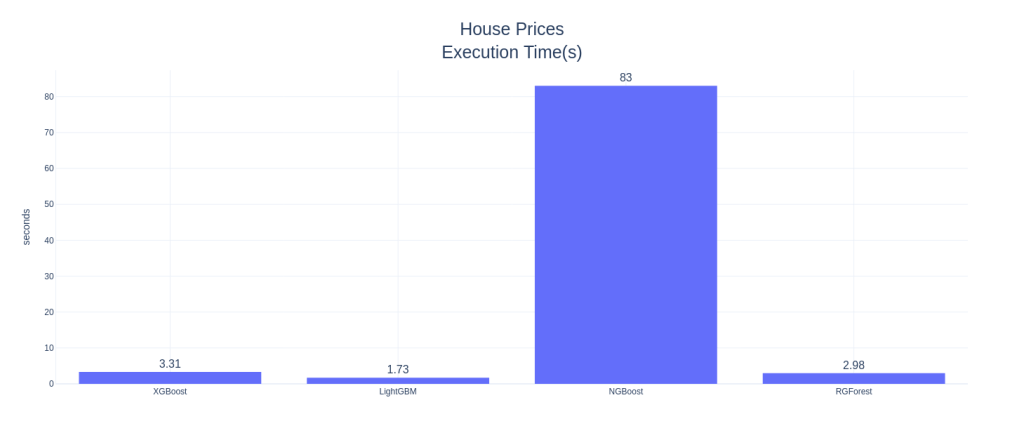
House Prices: Advanced Regression Techniques
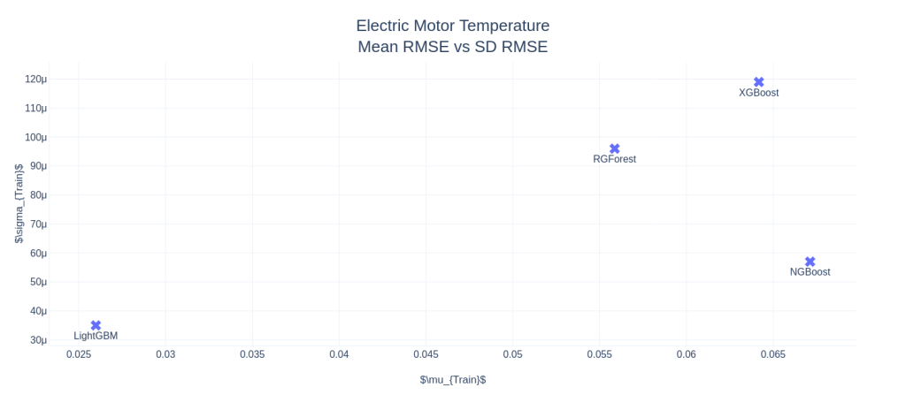
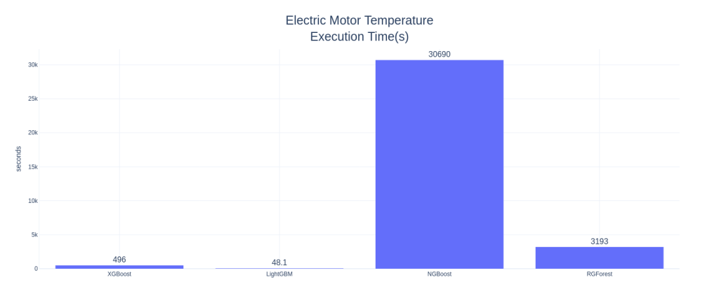
Electric Motor Temperature
Final Words
Disclaimer: These experiments are in no way complete. One would need a much larger scale experiment to arrive at a conclusion on which algorithm is doing better. And then there is the No Free Lunch Theorem to keep in mind.
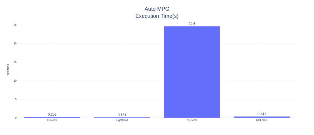
Right off the bat, NGBoost seems like a strong contender in this space. In AutoMPG and Housing Prices datasets, NGBoost performs the best among all the other boosters, both on mean RMSE as well as the Standard Deviation in the CV scores, and by a large margin. NGBoost also shows quite a large gap between the default and tuned versions. This shows that either the default parameters are not well set, or that each tuning for dataset is a key element in getting good performance from NGBoost. But the Achilles heel of the algorithm is the run-time. With those huge bars towering over the others, we can see that the runtime, really, is in a different scale as compared to the other boosters. Especially on large datasets like Electric Motors Temperature dataset, the runtime is prohibitively large and because of that I didn’t tune the algorithm as well. It fares last among the other boosters in the competition.
Another standout algorithm is Regularized Greedy Forest, which is performing as good as or even better than XGBoost. In low and medium data setting, the runtime is also comparable to the reigning king, XGBoost.
In low data setting, popular algorithms like XGBoost and LightGBM are not performing well. And the standard deviation of the CV scores are higher, especially XGBoost, showing that it overfits. XGBoost has this problem in all three examples. In the matter of runtime, LightGBM reins king(although I haven’t tuned for computational performance), beating XGBoost in all three examples. In the high data setting, it blew everything else out of the water by having much lower RMSE and runtime than the rest of the competitors.
colab Notebooks with experiments
We have come far and wide in the world of gradient boosting and I hope that at least for some of you, Gradient Boosting does not mean XGBoost. There are so many algorithms with its own quirks in this world and lot of them perform at par or better than XGBoost. And another exciting area is Probabilistic Regression. I hope NGBoost become more efficient and step over that hurdle of computational efficiency. Once that happens, NGBoost is a very strong candidate in the probabilistic regression space.
- Part I – Gradient boosting Algorithm
- Part II – Regularized Greedy Forest
- Part III – XGBoost
- Part IV – LightGBM
- Part V – CatBoost
- Part VI(A) – Natural Gradient
- Part VI(B) – NGBoost
- Part VII – The Battle of the Boosters
