Neural Oblivious Decision Ensembles(NODE) – A State-of-the-Art Deep Learning Algorithm for Tabular Data

Deep Learning brought about revolutions in many machine learning problems from the field of Computer Vision, Natural Language Processing, Reinforcement Learning, etc. But tabular data still remains firmly under classical machine learning algorithms, namely the gradient boosting algorithms(I have a whole series on different Gradient Boosting algorithms, if you are interested).

Intuitively, this is strange, isn’t it? Neural networks are universal approximators and ideally, they should be able to approximate the function even in the tabular data domain. Or may be they can, but need humungous amount of data to properly learn that function? But how does the Gradient Boosted Trees do it so well? May the inductive bias of a decision tree is well suited for tabular data domain?

If they are so good, why don’t we use decision trees in neural networks? Just like we have Convolution Operation for images, and Recurrent Networks for Text, why can’t we use Decision Trees as a basic building block for Tabular data?

The answer is pretty straightforward- Trees are not differentiable and without the gradients flowing through the network, back-prop bombs. But this is where researchers started to bang their heads. How do we make Decision Trees differentiable.

Differentiable Decision Trees

In 2015, Kontschieder et al., presented Deep Neural Decision Forests[1], which had a decision tree-like structure, but differentiable.

Let’s take a step back and think about a Decision Tree.

A typical Decision Tree looks something like the picture above. Simplistically, it is a collection of decision nodes( $d_i$ ) and leaf nodes( $\pi_i$ ) which together acts as a function,

$y = \mathcal{F}(\theta, X)$ , where $\mathcal{F}$ is the decision tree, parametrized by $\theta$ , which maps input $X$ to output $y$ .

Let’s look at the leaf nodes first, because it’s easier. In traditional Decision Trees, the leaf nodes is typically a distribution over the class labels. This is right up the alley of a Sigmoid or a Softmax activation. So we could really replace the leaf nodes with a SoftMax layer and make that node differentiable.

Now, let’s take a deeper look at a decision node. The core purpose of a decision node is to decide whether to route the sample to the left or right. Let’s call these decisions, $d_i \text{ and } \bar{d_i}$ . And for this decision, it uses a particular feature( $f$ ) and a threshold( $b$ )- these are the parameters of the node.

In traditional Decision Trees, this decision is a binary decision; it’s either right or left, 0 or 1. But this is deterministic and not differentiable. Now, what if we relax this and make the routing stochastic. Instead of a sharp 1 or 0, it’s going to be a number between 0 and 1. This feels like familiar territory, doesn’t it? Sigmoid function?

That’s exactly what Kontschieder et al. proposed. If we relax the strict 0-1 decision to a stochastic one with a sigmoid function, the node becomes differentiable.

Now we know how a single node(decision or a leaf node) works. Let’s put them all together. The red path in the diagram above is one of the path in the decision tree. In the deterministic version, a sample either goes through this route or it doesn’t. If we think about the same process in probabilistic terms, we know that the probability of the sample to go in the path should be 1 for every node in that path for the sample to reach the leaf node at the end of the path.

In the probabilistic paradigm, we find the probability that a sample goes left or right( $d_i \text{ and } \bar{d_i}$ ) and multiply all of those along the path to get the probability that a sample reaches the leaf node.

Probability of the sample reaching the highlighted leaf node would be ( $d_1 \cdot \bar{d_2} \cdot \bar{d_5}$ ).

Now, we just need to take the expected value of all the leaf nodes using the probabilities of each of the decision paths to get the prediction for a sample.

Now that you’ve got an intuition about how Decision Tree-like structures were derived to be used in Neural Networks, let’s talk about the NODE model[3].

Neural Oblivious Trees

An Oblivious Tree is a decision tree which is grown symmetrically. These are trees the same features are responsible in splitting learning instances into the left and the right partitions for each level of the tree. CatBoost, a prominent gradient boosting implementation, uses oblivious trees. Oblivious Trees are particularly interesting because they can be reduced to a Decision Table with $2^d$ cells, where $d$ is the depth of the tree. This simplifies things up pretty neatly.

Each Oblivious Decision Tree(ODT) outputs one of $2^d$ responses, where $d$ is the depth of the tree. This is done by using $d$ feature-threshold combinations, which are the parameters of the ODT.

Formally, the ODT can be defined as :

$h(x) = R[\mathbb{I}(f_1(x)-b_1), ..., \mathbb{I}(f_d(x)-b_d)]$ , where $\mathbb{I}$ denotes the Heaviside function(which is a step function which is 0 for negative or 1 for positive)

Now to make the tree output differentiable, we should replace the splitting feature choice( $f$ ) and the comparison operator using the threshold( $b$ ), but their continuous counterparts.

In Traditional Trees, the choice of a feature to split a node by is a deterministic decision. But for differentiability, we choose a softer approach, i.e. A weighted sum of the features, where the weights are learned. Normally, we would think of a Softmax choice over the features, but we want to have sparse feature selection, i.e. we want the decision to be made on only a handful(preferably 1) features. So, to that effect, NODE uses $\alpha$ -entmax transformation (Peters et al., 2019) over a learnable feature selection matrix $F \epsilon \mathcal{R}^{d \times n}$

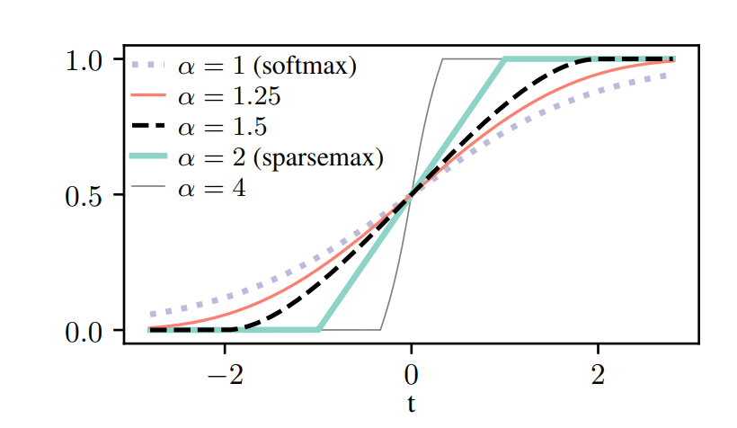
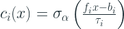
Similarly, we relax the Heaviside function as a two-class entmax. As different features can have different characteristic scales, we scale the entmax with a parameter $\tau$

$c_i(x) = \sigma_{\alpha}\left( \frac{f_i{x}-b_i}{\tau_i} \right )$ , where $b_i$ and $\tau_i$ are learnable parameters for thresholds and scales respectively.

We know that a tree has two sides and by $c_i$ , we have only defined one side. So to complete the tree, we stack $c_i \text{ and } (1-c_i)$ one on top of the other. Now we define a “choice” tensor $C$ as the outer product of all the trees:

$C(x) = \begin{bmatrix} c_1(x)) \\ 1-c_1(x) \end{bmatrix}\bigotimes \begin{bmatrix} c_2(x)) \\ 1-c_2(x) \end{bmatrix} \bigotimes ... \bigotimes \begin{bmatrix} c_d(x)) \\ 1-c_d(x) \end{bmatrix}$

This gives us the choice weights, or intuitively the probabilities of each of the $2^d$ outputs, which is in the Response tensor. So now it reduced into a weighted sum of Response tensor, weighted by the Choice tensor.

$h(x)= \sum_{i_i, . . . i_d \epsilon /{0,1/}^d} R_{i_i, . . . i_d} \cdot C{i_i, . . . i_d}(x)$

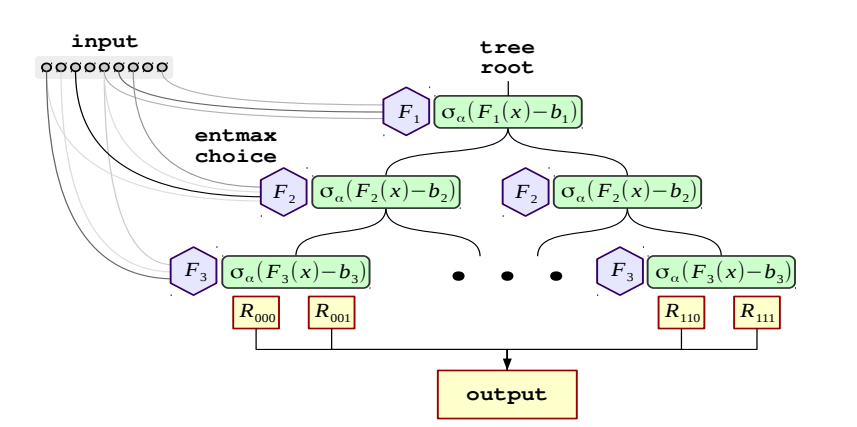
The entire setup looks like the below diagram:

Neural Oblivious Decision Ensembles

The jump from an individual tree to a “forest” is pretty simple. If we have $m$ trees in the ensemble, the final output is the concatenation of m individual trees $\left[ \hat{h_1}(x), . . . , \hat{h_m}(x) \right]$

Going Deeper with NODE

In addition to developing the core module(NODE layer), they also propose a deep version, where we stack multiple NODE layers on top of each other, but with residual connections. The input features and the outputs of all previous layers are concatenated and fed into the next NODE Layer and so on. And finally, the final output from all the layers are averaged(similar to the RandomForest).

Training and Experiments

Data Processing

In all the experiments in the paper[3], they transformed each of the features to follow a normal distribution using a Quantile Transformation. This step was important for stable training and faster convergence.

Initialization

Before training the network, they propose to do data-aware initialization to get good initial parameters. They initialize the Feature Selection matrix( $F$ ) uniformly, while the thresholds( $b$ ) are initialize with random feature values $f_i(x)$ . The scales $\tau_i$ are initialize in such a way that all the samples in he first batch fall in the linear region of the $latex two-sided entmax and hence receive non-zero gradients. And finally, the response tensor are initialized with a standard normal distribution.

Experiments and Results

The paper performs experiments with 6 datasets – Epsilon, YearPrediction, Higgs, Microsoft, Yahoo, and Click. They compared NODE with CatBoost, XGBoost and FCNN.

First they compared with default hyperparameters across all the algorithms. the default architecture of NODE was set as below: Single layer of 2048 trees of depth 6. These parameters were inherited from CatBoost default parameters.

Then, they tuned all the algorithms and then compared.

Code and Implementation

The authors have made the implementation available in a ready to use Module in PyTorch here.

It is also implemented in the new library I released, PyTorch Tabular, along with a few other State of the Art algorithms for Tabular data. Check it out here:

References

P. Kontschieder, M. Fiterau, A. Criminisi and S. R. Bulò, “Deep Neural Decision Forests,” 2015 IEEE International Conference on Computer Vision (ICCV), pp. 1467-1475, doi: 10.1109/ICCV.2015.172.
Ben Peters, Vlad Niculae, André F. T. Martins, “Sparse Sequence-to-Sequence Models,” 2019 Proceedings of the 57th Annual Meeting of the Association for Computational Linguistics(ACL), pp. 1504-1519, doi: 10.18653/v1/P19-1146.
Sergei Popov, Stanislav Morozov, Artem Babenko, “Neural Oblivious Decision Ensembles for Deep Learning on Tabular Data,” arXiv:1909.06312 [cs.LG]

Neural Oblivious Decision Ensembles(NODE) – A State-of-the-Art Deep Learning Algorithm for Tabular Data

Differentiable Decision Trees

Neural Oblivious Trees

Neural Oblivious Decision Ensembles

Going Deeper with NODE