Time Series Imputation using Matrix Recovery

Missing values in time series are not straightforward to deal with. In my book on time series forecasting, Modern Time Series Forecasting with Python, I talk about a few techniques, right from thinking about the missing values in the right way to some algorithmic techniques to deal with missing data (like seasonal interpolation).

Originally, that discussion was supposed to be longer and also included a few advanced matrix recovery based techniques which is really useful in related datasets. What if we can use the information of other related time series to help fill in the gaps in an intelligent way? But because of the fact that the book was already getting too big, we had to edit some of these out.

Here, I reproduce the part of the book that was omitted from the book. If you have bought the book, this will be an extension to what you already have. The code used and implementations are already part of the Github repo. The data used for the code examples are also the same as the one in the book. If you haven’t, then I suggest you do that 😋. But seriously, even if you haven’t bought the book, the Github repo is public and instructions to download the data and setup the environment are already there in the Readme.

Now, on to the part which was omitted from the book:

Matrix Recovery Techniques

Matrix recovery techniques which are widely used in Recommendation Systems, where we hope to complete the user-item interaction matrix so that we can recommend better items to users. But these techniques are widely used in other domains as well, and one of those uses is to impute missing values in datasets. Instead of looking at each timeseries in isolation, this family of methods rely on a group of related time series to fill in the missing data.

The key idea is this: we assume that there exists a low-rank matrix which can faithfully represent the information in the larger matrix, and we try to find that matrix.

Additional Information
The rank of a matrix is the maximum number of its linearly independent column vectors or row vectors. From the definition, we know that it is always less than or equal to the number of columns (or rows) in a matrix. If any column (or row) in a matrix is a linear combination of any other columns (or rows), we say that the matrix is not full-rank. Rank of the matrix can also be found out by doing a Singular Value Decomposition of the matrix and counting the non-zero eigen values.

We can formulate this as a learning problem where we learn a matrix $Z_{m \times n}$ :

$\text{minimize. }rank(Z)$

$\text{subject to }\sum_{(i,j) \in \Phi}(X_{ij} - Z_{ ij})^2 <= \delta$

where $\delta$ is a regularization parameter controlling the tolerance in training error. But the minimization of rank is intractable and therefore we have many alternates or heuristics to solve this optimization problem.

Since we need a set of related time series to carry out matrix recovery based techniques let’s prepare a dataframe with all the time series in the block, the different timeseries forming the different columns in the dataframe.

all_ts_df = pd.pivot_table(exp_block_df, 
    index="timestamp", 
    columns="LCLid",
    values="energy_consumption"
)
# Nulling out the window
all_ts_df.loc[window, "MAC000193"] = np.nan

Now we will go through a few of the matrix recovery techniques:

Matrix Factorization

Let’s understand the concept using an example from Recommendation Systems, (because it’s easier to understand), and then extend the intuition to time series.

The user-item matrix in Recommendation Systems is a matrix which has the users along the rows and items (let’s say movies) along the columns. At the intersection of a user and an item, we have the rating of the user for that item. If we have $N$ users and $M$ items, we have an interaction matrix $\mathbf{I}$ of $N \times M$ . We assume that each user and item can be represented by a set of $r$ attributes, where $r$ is much smaller than the original size of the matrix. This is possible because there exists dominant correlations among the columns and rows of the matrix.

Even though we like to believe that each of us are unique in our taste of movies, we still can be grouped together with other users who like the same stuff we do. Similarly, items can also be grouped together based on similarities between them. So, through matrix factorization, we decompose our user-item matrix into two matrices, $\mathbf{U}_{N \times r}$ and $\mathbf{V}_{r \times M}$ such that, $\mathbf{U}^T \times \mathbf{V} = \mathbf{I}$ . The matrix $\mathbf{U}$ is called the user latent factors and matrix $\mathbf{V}$ is called the Item latent factors.

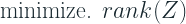
Now let’s switch our attention towards set of related time series. We have a set of $N$ time series with $L$ timesteps, which gives us the interaction matrix $\mathbf{Y}$ of size $N \times L$ . Like the user-item matrix, this matrix also has dominant correlations, i.e., there are a smaller set of patterns which can describe the matrix. Some timeseries will behave similarly. Maybe with a fixed trend, or with strong seasonality. And some timesteps will also share common patterns, such as the increase in energy consumption because of a public holiday or because of weekends. So, when we apply matrix factorization to such a matrix, what we get is again two matrices, $\mathbf{U}_{N \times r}$ and $\mathbf{V}_{r \times L}$ such that, $\mathbf{U}^T \times \mathbf{V} = \mathbf{Y}$ . The matrix $\mathbf{U}$ has latent factors which are related to the temporal aspect and the matrix $\mathbf{V}$ has latent factors specific to individual timeseries. The below diagram illustrates the process visually.

Fig 2.11: Matrix Factorization of set of related time series

But how do we get these matrices? This is where gradient descent steps in. We can learn these matrices is using a loss (either L1, L2, or any other regression loss) on the observed values leveraging gradient descent. Once we have these matrices, we have a way of recovering the missing data by multiplying the two together.

We will be using the python library fancyimpute for this exercise. It has a lot of matrix recovery techniques implemented and we can use it with an API that is similar to scikit-learn.

from fancyimpute import MatrixFactorization
recovered_matrix_mf = MatrixFactorization(
    rank=50
).fit_transform(all_ts_df.values)

The rank of the matrix is a hyperparameter and we will need to find with a good cross validation setup. For the exercise, we have just done a simple Grid Search with the artificially created timeseries gap as the test set. Let’s see how the recovery looks like.

Fig 2.12: Imputing with Matrix Factorization

We can see that the seasonal profile has been captured in the imputed time series, but the MAE is slightly on the higher side.

Truncated Singular Value Decomposition and Iterative Singular Value Decomposition

Another way to calculate the decomposed matrices is using Singular Value Decomposition(SVD). SVD is a technique by which we factorize any real matrix into singular matrices and singular values. The SVD can be represented as the equation below, where $\mathbf{A}$ is the original matrix, $\mathbf{U}$ is the left singular matrix, $\mathbf{V}$ is the right singular matrix and $\mathbf{D}$ is a diagonal matrix with the number of singular values(r).

$A \approx \mathbf{U} \times \mathbf{D} \times \mathbf{V}^T$

The singular values in $\mathbf{D}$ , is arranged in such a way that the highest value occurs at the top of the diagonal, and it decreases as we move down the diagonal. The dimensions of $\mathbf{U}$ and $\mathbf{V}$ is such that the matrix multiplication gives you back the original matrix.

The figure below depicts an SVD visually:

If you’ve heard about Principal Component Analysis(PCA), this procedure has strong connections with it. The singular values can be considered similar to the eigenvalues that you get from PCA.

There are many ways of performing an SVD but we won’t be going into those because it is out of scope for this book. But popular libraries like numpy and scipy has implementations that we can use for this purpose.

While this looks straightforward, there is a problem. SVD doesn’t work on incomplete matrices. So, if we have missing values, it needs to be filled in with something before doing the SVD. This kind of defeats the purpose, doesn’t it? One way is to fill in with zeroes or mean or some kind of approximation, carry out the SVD, and then use the resulting matrices to recover missing values in our data. But what this would do is give you back the same approximation you used to fill in the missing values back as the result.

This is where Truncated SVD comes in. Truncated SVD makes the assumption that we do not need all the singular values to reconstruct the matrix. Instead, it chooses ${r}'$ highest singular values and only use those to reconstruct the matrix. When we are using ${r}'$ singular values, we will also be only using the first ${r}'$ columns from $\mathbf{U}$ and $\mathbf{V}$ to carry out the matrix multiplication required to recover the original matrix $\mathbf{A}$ .

The below figure illustrates this process.

Fig 2.14: Truncated Singular Value Decomposition

What this allows us to do is extract the key patterns in the data and use it to reconstruct the missing data. So the approximation we used to fill in the initial matrix can be ignored in favor of the dominant patterns in the data while reconstructing the matrix.

Let’s see this is action. We have implemented this recovery technique in the associated Github repository at src/imputation/matrix_recovery.py. We can use it like below.

from src.imputation.truncated_svd import TruncatedSVDImputation
recovered_matrix_tsvd = TruncatedSVDImputation(
    rank=2, 
    init_fill_method="zero", 
    min_value=0
).fit_transform(all_ts_df.values)

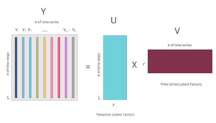
Let’s see how this imputation worked.

Fig 2.15: Imputing with Truncated Singular Value Decomposition

The seasonal pattern has been captured but is slightly off with a peak at 6 PM the first day. We can see that the MAE is also not that great.

Iterative SVD is another heuristic which tries to overcome the inaccuracies that arises out of the initial filling of missing values before SVD. In Iterative SVD, we do this Truncated SVD multiple times, each iteration replacing the missing values with the imputed values. We start off by imputing the missing values with zero, mean or some other approximations and run the truncated SVD to recover the missing values. Then the approximations we had earlier on is replaced with the new missing values and truncated SVD is run again. This process is continued either till we reach maximum iterations or a convergence criterion.

This is already implemented in fancyimpute and we are going to use that.

from fancyimpute import IterativeSVD
recovered_matrix_isvd = IterativeSVD(
    rank=2, 
    max_iters=1000, 
    svd_algorithm="arpack", 
    min_value=0
).fit_transform(all_ts_df.values)

The key hyperparameter here is the rank which, similar to matrix factorization, we need to find by using a good cross validation framework. If the matrix you are handling is very large, passing svd_algorithm = “randomized” as a parameter carries out Randomized SVD, which is a faster approximation of the SVD.

Let’s see how this technique fared:

Fig 2.16: Imputing with Iterative Singular Value Decomposition

The pattern captured is almost identical to the simple Truncated SVD with similar MAE.

Soft Impute

Soft Impute is another technique which has SVD at the heart of it. In 2010, Rahul Mazumder et.al. presented a paper named Spectral Regularization Algorithms for Learning Large Incomplete Matrices^[1]. It is a heuristic similar to Iterative SVD, but instead of using a fixed rank in each iteration, the algorithm uses a thresholding technique to select the important singular values to be used. We have a parameter called shrinkage which determines how much of the singular values are “shrinked” in each iteration. fancyimpute has an implementation of this algorithm, which we can use. Let’s see how that is done.

recovered_matrix_si = SoftImpute(
    shrinkage_value=70, 
    max_iters=1000, 
    min_value=0
).fit_transform(all_ts_df.values)

Instead of tuning the rank, the key hyperparameter here is the shrinkage_value. By default the implementation uses 1/50^th of the maximum singular value as the shrinkage_value. But we can define our own grid and search for best values in that grid. To do that, we just need to look at the top 10 singular values and define a range according to those values.

from sklearn.utils.extmath import randomized_svd
# quick decomposition of X_filled into rank-1 SVD
_, s, _ = randomized_svd(
    all_ts_df.fillna(0).values,
    10,
    n_iter=5)
print(f"The Singular Values are: {s}")
>> The Singular Values are: 
[449.19968819 226.76815429 108.13701595 104.16274052  
93.04365049  84.55941487  75.96773552  73.72644566  
67.74005664  64.71221699]

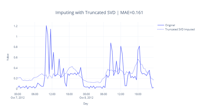
In this case we defined the grid as [60, 70, 80, 90, 100, 150, 250], found that shrinkage_value=70 gives us lowest reconstruction error, and used that shrinkage value in the recovery algorithm. Let’s see how this looks like:

We can see that this is slightly better in capturing the lows around midnight and early mornings and hence has lower MAE as well.

Centroid Recovery

Centroid Decomposition is an approximation for SVD. It computes centroid values, loading vectors, relevance vectors approximating singular values, right singular matrix and left singular matrix of the SVD respectively. The centroid decomposition of a $m \times n$ matrix $\mathbf{A}$ is of the form $\mathbf{A} \approx \mathbf{L} \times \mathbf{R}^T$ where $\mathbf{L}$ is an $m \times n$ matrix and $\mathbf{R}$ is a $n \times n$ matrix. But similar to truncated SVD, in Centroid Decomposition also we truncate the resulting matrices to $r << n$ while reconstructing the original matrix. Classical approaches to Centroid Decomposition are brute force driven and for large matrices becomes prohibitive in both space and time complexities.

Khayati, M et.al. proposed a scalable algorithm^[2] to calculate Centroid Decomposition, which can be used for matrix recovery. We have implemented this recovery technique in the associated Github repository at src/imputation/matrix_recovery.py. We can use it like below.

from src.imputation.cdrec import CentroidRecovery
recovered_matrix_cdrec = CentroidRecovery(
    truncation=5, 
    max_iters=100, 
    init_fill_method="interpolate", 
    min_value=0, 
    early_stopping=True
).fit_transform(all_ts_df.values)

The key parameter here is again similar to rank: truncation. It determines how much of a reduction in rank are we enforcing while generating the factorized matrices. As always, we find it using something like a grid search with a strong cross validation setup. Let’s see how it does:

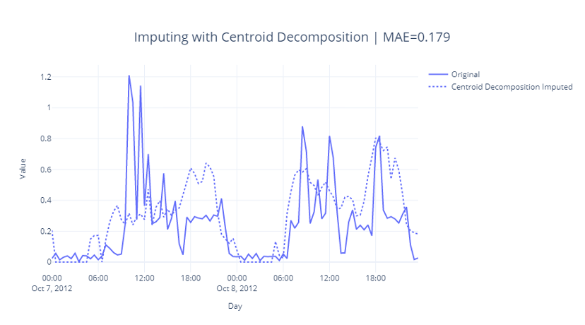
Fig 2.17: Imputing with Centroid Decomposition

References

Mazumder, Rahul & Hastie, Trevor & Tibshirani, Robert. (2010). Spectral Regularization Algorithms for Learning Large Incomplete Matrices. Journal of machine learning research : JMLR. 11. 2287-2322. – https://www.jmlr.org/papers/v11/mazumder10a.html
Khayati, M., Cudré-Mauroux, P. & Böhlen, M.H. Scalable recovery of missing blocks in time series with high and low cross-correlations. Knowl Inf Syst 62, 2257–2280 (2020). https://doi.org/10.1007/s10115-019-01421-7

Time Series Imputation using Matrix Recovery

Matrix Recovery Techniques

Matrix Factorization

Truncated Singular Value Decomposition and Iterative Singular Value Decomposition

Soft Impute

Centroid Recovery

References

Further Reading

Modern Time Series Forecasting with Python

Published by Manu Joseph

Leave a Reply Cancel reply

Time Series Imputation using Matrix Recovery

Matrix Recovery Techniques

Matrix Factorization

Truncated Singular Value Decomposition and Iterative Singular Value Decomposition

Soft Impute

Centroid Recovery

References

Further Reading

Modern Time Series Forecasting with Python

Share this:

Like this:

Related

Published by Manu Joseph

Leave a Reply Cancel reply