Mixture Density Networks: Probabilistic Regression for Uncertainty Estimation

Uncertainty is all around us. It is present in every decision we make, every action we take. And this is especially true in business decisions where we plan for the future. But in spite of that, all of our predictive models that we use in business ignore uncertainty.

Suppose you are the manager of the Google Play Store and Google Pixel 5a launch is coming up. HQ sends you a forecast from their ML model and says that they expect 100 units to be sold in the first week of launch. But you know, from you experience, that the HQ predictions are not always right and want to hedge against a stock out by procuring more than 100. But how much more? How do you know how wrong the prediction from the ML model will be? In other words, how confident this prediction of a 100 units is? This additional information of the confidence of the model is crucial in making this decision and the ML model from HQ does not give you that. But what if in addition to this forecast of 100 units, the model also gives you a measure of uncertainty– like the standard deviation of the expected probability distribution? Now you can make an informed decision based on your risk appetite on how much to over-stock.

But how do we do that? Usually, classification problems have an added advantage because of the logistic function we slap on at the top which gives us some idea about the confidence of the model(although it is not technically the same thing). When it comes to regression, our traditional models gives us a point estimate.

Types of Uncertainty

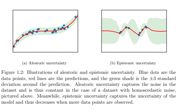
There are two major kinds of uncertainty – Epistemic and Aleatoric Uncertainty (phew, that was quite a mouthful).

• Epistemic Uncertainty describes what the model doesn’t know. It is attributed to inadequate knowledge of the model. This is the uncertainty which can be reduced by having more data or increasing the model complexity.
• Aleatoric Uncertainty is the inherent uncertainty which is part of the data generating process. For example, a paper plane which is launched by a high precision equipment, which maintains the same degree of release, speed of release and a thousand other parameters will still not fall in the same place each trial. This inherent variability is Aleatoric Uncertainty.

A typical supervised machine learning problem can be written as below:

Here the epistemic uncertainty is derived from and the aleatoric from . Typically high epistemic uncertainty is found in the part of the feature space which is sparsely populated with data examples. In such an n-dimensional space, there might be many parameters which can explain the given data points and this leads to uncertainty.

The Core Idea

The key innovation here is like this:

In a vanilla Neural Network regression, we will have a single neuron at the last layer which is trained to predict the value that we are interested in. What if we predict the parameters of a probability distribution instead? For example, a Gaussian distribution is parametrized by its mean() and its standard deviation(). So instead of having a single neuron in the last layer, we have two which predicts the mean and the standard deviation of the Gaussian Distribution.

Awesome! When properly trained, we have the mean and the standard deviation, which means we have the entire probability distribution and therefore by extension as estimate of the uncertainty.

But, there is a problem. When we train the model to predict the parameters of the distribution, we are slapping on a huge inductive bias onto the model. for all we know, the target variable that we are trying to model might not even follow any parametric distribution.

Let’s look at the bimodal example. It looks like there are two gaussian distributions, squished together. And if we do a though experiment, and extend this “squishing of two gaussian distributions” to “squishing of N gaussian distributions“, this resultant mixture can model a wide variety of probability distributions. This is exactly the code idea of a Mixture Density network is. You have a number of gaussian components(mean and standard deviation) which comprises the last layer in the network. And have another learned parameter(a latent representation) which decides how to mix these gaussian components.

Mixture Density Networks

Mixture Density Networks are built from two components – a Neural Network and a Mixture Model.

The Neural Network can be any valid architecture which takes in the input and converts into a set of learned features(we can think of it as an encoder or backbone).

Now, let’s take a look at the Mixture Model. The Mixture Model, like we discussed before, is a model of probability distributions built up with a weighted sum of more simple distributions. More formally, it models a probability density function(pdf) as a mixture of m pdfs indexed by j , with weights by the following equation:

, where are the parameters of the distribution describing the shape and location of the distribution.

In his paper[1], Bishop uses the Gaussian kernel and explains that any probability density function can be approximated to arbitrary accuracy, provided the mixing coefficients and the Gaussian parameters are correctly chosen. By using the Gaussian kernel in the above equation. it becomes:

Sufficient Conditions

Bishop proposed a few restrictions and ways to implement the MDNs as well.

1. The mixing coefficients () are probabilities and have to be less than one and sum to unity. This can be easily achieved by passing the outputs of the mixing coefficients through a Softmax layer.
2. The variance () should be strictly positive. Bishop[1] suggested that we use the exponential function to the raw logits of the sigma neuron. He suggested that this had the same effect as assuming an uninformative prior and avoids the pathological configurations in which one or more of the variances goes to zero.
3. The center parameters () represent location parameters and this should be the raw logits of the mean neuron.

Loss Function

The network is trained end-to-end using standard backpropagation. And for that the loss function we are minimizing is the Negative Log Likelihood, which is equivalent to the Maximum Likelihood Estimation.

We already know what is and it’s just the matter of calculating it and maximizing the negative log-likelihood.

Implementation & Tricks to Ensure Stability

Now that we know the theory behind the model, let’s look at how we can implement it(and a few tricks and failure modes). Implementing and training an MDN is notoriously hard because there are just a lot of things that could go wrong. But through adopting prior research and a lot of experimentation, I have fixed on a few tricks which makes the training relatively stable. The implementation will be in PyTorch using a library that I developed – Pytorch Tabular(which is a highly flexible framework to work with deep learning and tabular data).

Avoiding Numerical Underflow

If you remember the pdf formula for the Gaussian mixture, it involves the summation of all the pdf‘s weighted by the mixing coefficients. So the Negative Log-Likelihood would be:

and we know that

If you examine the equation, we see an exponential function which is then multiplied with the mixing coefficients and then take the log of it. This exponential and the subsequent log can lead to very small numbers leading to numerical underflow. So we as suggested by Axel Brando Guillaumes [3] use the LogsumExp trick and carry out the calculations in log domain.

So the negative log likelihood becomes:

Now using the torch.logsumexp we calculate the negative log-likelihood of all the samples in the batch and then compute the mean. This helps us avoid a lot of numerical instabilities in training.

The Activation Function for Variance Parameter

Bishop[1] suggested to use an Exponential activation function for the variance parameter. The choice has its strengths. The exponential function tends to a positive output and on the lower side, it never really reaches zero. But practically, it has some problems. The exponential function grows very large very fast and in case of datasets with high variance, the training becomes unstable.

Axel Brando Guillaumes [3] proposes an alternative, which is what we have used in our implementation. A modified version of an ELU activation.

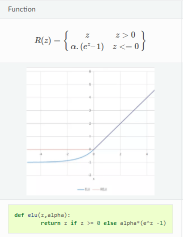
The ELU function retains the exponential behavior and reverts to a linear behavior for higher values. The only problem is that the exponential behavior is when x is negative. But if we move this function upwards by 1, we have a function which approximates the exponential behavior. So Axel Brando Guillaumes [3] proposed to use 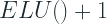as the activation function for the variance parameter. Since technically this also can become zero, we have added an epsilon also to the modified ELU to ensure stability. So the final activation used is:

Multiple Gaussians and Mode Collapse

When we are using multiple Gaussian components and training the model using backpropagation, there is a tendency for the network to ignore all but one of the components and train a single component to explain the data. For eg. if we are using two components, while training one component will tend to zero and the other to 1 and the mean and variance components corresponding to the mixing component which became 1 will be trained to explain the data.

Axel Brando Guillaumes [3] suggests to clip the value to a lower limit. But there was a problem with this approach.

• Because of the softmax applied, you can’t clip the after applying softmax; otherwise it won’t add up to one. And before softmax, you have to apply the clipping on the raw logit value, which is highly unintuitive.

So, through experimentation, we found out another set of tricks to make the network behave(although not guaranteed, but certainly encourage the network away from mode collapse).

1. Weight Regularization – Applying L1 or L2 regularization to the weights of the neurons which compute the mean, variances and mixing components.
2. Bias Initialization – If we precompute the possible centers of the two gaussians, we can initialize the bias of the layers to these centers. This has shown to have a strong effect in the separation of the two gaussian kernels/components during training.

Alternative for Softmax for Mixing Coefficients

Bishop[1] suggested to use a Softmax layer to convert the raw logits of the mixing coefficients() to probabilities. But we have used a Gumbel Softmax, which provides a much more sharper probability distribution. This is desirable because we want our model to be able to efficiently factor out one or more components when it is not needed. Softmax would still assign a small probability to those, while Gumbel Softmax makes that probability even smaller.

Code

Below is a sample code for the implementation in PyTorch Tabular. Head over to the repo to see the full implementation(as a bonus also have access to implementations to other models like NODE, AutoInt, etc as well).

	#Sample Implementation for educational purposes
	#For full implementation check out https://github.com/manujosephv/pytorch_tabular
	ONEOVERSQRT2PI = 1.0 / math.sqrt(2 * math.pi)
	LOG2PI = math.log(2 * math.pi)
	class MixtureDensityHead(nn.Module):
	def __init__(self, config: DictConfig, **kwargs):
	self.hparams = config
	super().__init__()
	self._build_network()
	def _build_network(self):
	self.pi = nn.Linear(self.hparams.input_dim, self.hparams.num_gaussian)
	nn.init.normal_(self.pi.weight)
	self.sigma = nn.Linear(
	self.hparams.input_dim,
	self.hparams.num_gaussian,
	bias=self.hparams.sigma_bias_flag,
	)
	self.mu = nn.Linear(self.hparams.input_dim, self.hparams.num_gaussian)
	nn.init.normal_(self.mu.weight)
	if self.hparams.mu_bias_init is not None:
	for i, bias in enumerate(self.hparams.mu_bias_init):
	nn.init.constant_(self.mu.bias[i], bias)
	def forward(self, x):
	pi = self.pi(x)
	sigma = self.sigma(x)
	# Applying modified ELU activation
	sigma = nn.ELU()(sigma) + 1 + 1e-15
	mu = self.mu(x)
	return pi, sigma, mu
	def gaussian_probability(self, sigma, mu, target, log=False):
	"""Returns the probability of `target` given MoG parameters `sigma` and `mu`.
	Arguments:
	sigma (BxGxO): The standard deviation of the Gaussians. B is the batch
	size, G is the number of Gaussians, and O is the number of
	dimensions per Gaussian.
	mu (BxGxO): The means of the Gaussians. B is the batch size, G is the
	number of Gaussians, and O is the number of dimensions per Gaussian.
	target (BxI): A batch of target. B is the batch size and I is the number of
	input dimensions.
	Returns:
	probabilities (BxG): The probability of each point in the probability
	of the distribution in the corresponding sigma/mu index.
	"""
	target = target.expand_as(sigma)
	if log:
	ret = (
	–torch.log(sigma)
	– 0.5 * LOG2PI
	– 0.5 * torch.pow((target – mu) / sigma, 2)
	)
	else:
	ret = (ONEOVERSQRT2PI / sigma) * torch.exp(
	–0.5 * ((target – mu) / sigma) ** 2
	)
	return ret # torch.prod(ret, 2)
	def log_prob(self, pi, sigma, mu, y):
	log_component_prob = self.gaussian_probability(sigma, mu, y, log=True)
	log_mix_prob = torch.log(
	nn.functional.gumbel_softmax(pi, tau=1, dim=–1) + 1e-15
	)
	return torch.logsumexp(log_component_prob + log_mix_prob, dim=–1)
	def sample(self, pi, sigma, mu):
	"""Draw samples from a MoG."""
	categorical = Categorical(pi)
	pis = categorical.sample().unsqueeze(1)
	sample = Variable(sigma.data.new(sigma.size(0), 1).normal_())
	# Gathering from the n Gaussian Distribution based on sampled indices
	sample = sample * sigma.gather(1, pis) + mu.gather(1, pis)
	return sample
	def generate_samples(self, pi, sigma, mu, n_samples=None):
	if n_samples is None:
	n_samples = self.hparams.n_samples
	samples = []
	softmax_pi = nn.functional.gumbel_softmax(pi, tau=1, dim=–1)
	assert (
	softmax_pi < 0
	).sum().item() == 0, "pi parameter should not have negative"
	for _ in range(n_samples):
	samples.append(self.sample(softmax_pi, sigma, mu))
	samples = torch.cat(samples, dim=1)
	return samples
	def generate_point_predictions(self, pi, sigma, mu, n_samples=None):
	# Sample using n_samples and take average
	samples = self.generate_samples(pi, sigma, mu, n_samples)
	if self.hparams.central_tendency == "mean":
	y_hat = torch.mean(samples, dim=–1)
	elif self.hparams.central_tendency == "median":
	y_hat = torch.median(samples, dim=–1).values
	return y_hat

view raw mdn_head.py hosted with ❤ by GitHub

	#Sample Implementation for educational purposes
	#For full implementation check out https://github.com/manujosephv/pytorch_tabular
	class BaseMDN(BaseModel):
	def __init__(self, config: DictConfig, **kwargs):
	super().__init__(config, **kwargs)
	@abstractmethod
	def unpack_input(self, x: Dict):
	pass
	def forward(self, x: Dict):
	x = self.unpack_input(x)
	x = self.backbone(x)
	pi, sigma, mu = self.mdn(x)
	return {"pi": pi, "sigma": sigma, "mu": mu, "backbone_features": x}
	def sample(self, x: Dict, n_samples: Optional[int] = None, ret_model_output = False):
	ret_value = self.forward(x)
	samples= self.mdn.generate_samples(
	ret_value["pi"], ret_value["sigma"], ret_value["mu"], n_samples
	)
	if ret_model_output:
	return samples, ret_value
	else:
	return samples
	def calculate_loss(self, y, pi, sigma, mu, tag="train"):
	# NLL Loss
	log_prob = self.mdn.log_prob(pi, sigma, mu, y)
	loss = torch.mean(–log_prob)
	if self.hparams.mdn_config.weight_regularization is not None:
	sigma_l1_reg = 0
	pi_l1_reg = 0
	mu_l1_reg = 0
	if self.hparams.mdn_config.lambda_sigma > 0:
	# Weight Regularization Sigma
	sigma_params = torch.cat(
	[x.view(–1) for x in self.mdn.sigma.parameters()]
	)
	sigma_l1_reg = self.hparams.mdn_config.lambda_sigma * torch.norm(
	sigma_params, self.hparams.mdn_config.weight_regularization
	)
	if self.hparams.mdn_config.lambda_pi > 0:
	pi_params = torch.cat([x.view(–1) for x in self.mdn.pi.parameters()])
	pi_l1_reg = self.hparams.mdn_config.lambda_sigma * torch.norm(
	pi_params, self.hparams.mdn_config.weight_regularization
	)
	if self.hparams.mdn_config.lambda_mu > 0:
	mu_params = torch.cat([x.view(–1) for x in self.mdn.mu.parameters()])
	mu_l1_reg = self.hparams.mdn_config.lambda_mu * torch.norm(
	mu_params, self.hparams.mdn_config.weight_regularization
	)
	loss = loss + sigma_l1_reg + pi_l1_reg + mu_l1_reg
	self.log(
	f"{tag}_loss",
	loss,
	on_epoch=(tag == "valid"),
	on_step=(tag == "train"),
	# on_step=False,
	logger=True,
	prog_bar=True,
	)
	return loss

view raw base_mdn.py hosted with ❤ by GitHub

Experiments

Taking inspiration from this excellent Colab Notebook by Dr. Oliver Borchers, I have designed my own set of experiments using the implementation. There is also a tutorial on how to use MDNs in PyTorch Tabular here.

Linear Function

This is a simple linear function, but some gaussian noise added as a function of the input x. A regular feedforward network will be able to approximate this function with a straight line through the middle. But if we use an MDN with a single component, it will approximate both the mean and the uncertainty in the function

Non-Linear Function

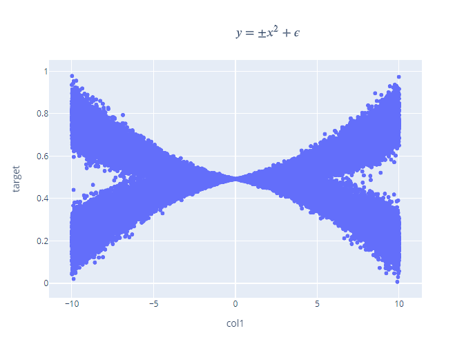
This is a non-linear function with a twist. For each value of x, there are two values of y – one of the positive side and another on the negative side. Let’s take a look at what happens if we fit a normal FeedForward network on this data.

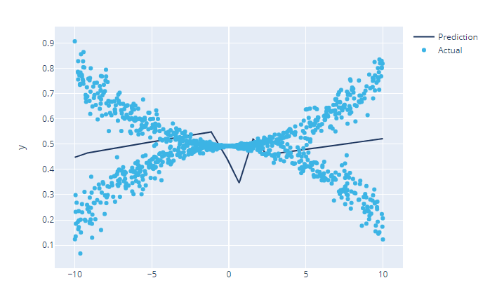
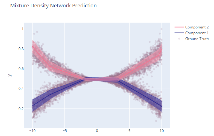
Not very good isn’t it? Well, if you think of the maximum likelihood estimate, it will likely fail because both the positive and negative points are equally likely. But when you train an MDN on it, the two components are properly learned and if we plot out the two components, it will look like this:

Gaussian Mixture

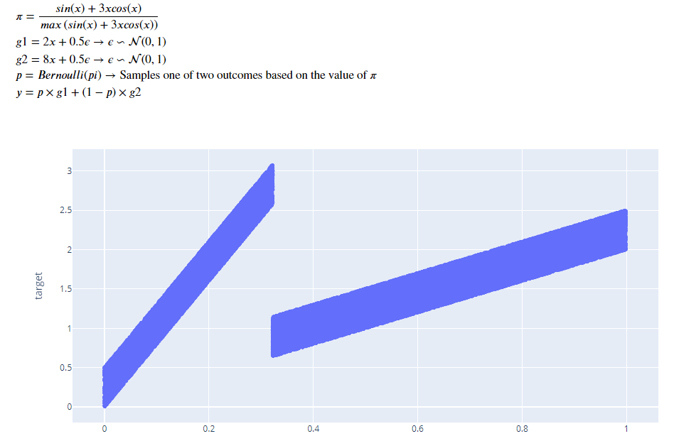
Here we have two gaussian components which are mixed in a ratio, all of which is parameterized by x.

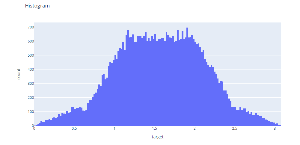
The histogram also shows two small bumps on the top instead of a single smooth on of a normal gaussian.

Let’s look at how the standard FeedForward network captures this function.

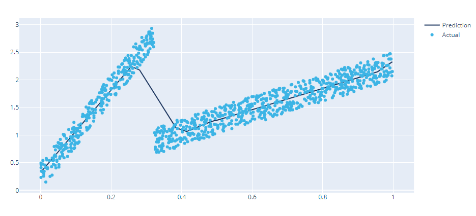
Pretty well, except for the part where there is a transition. And as always no information about the uncertainty. (note: Really awesome how the network bends itself to approximate the step function.

Now let’s train an MDN on this data.

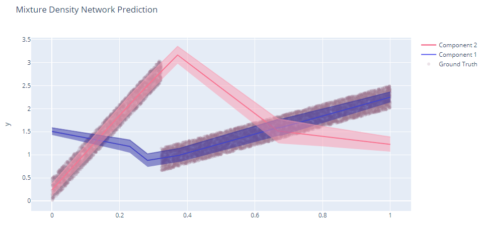
Now, isn’t that something? The two components are well captured – one component captures the first part well and the other one does the second one. The uncertainty is also estimated pretty well. Let’s also take a look at the mixing coefficients.

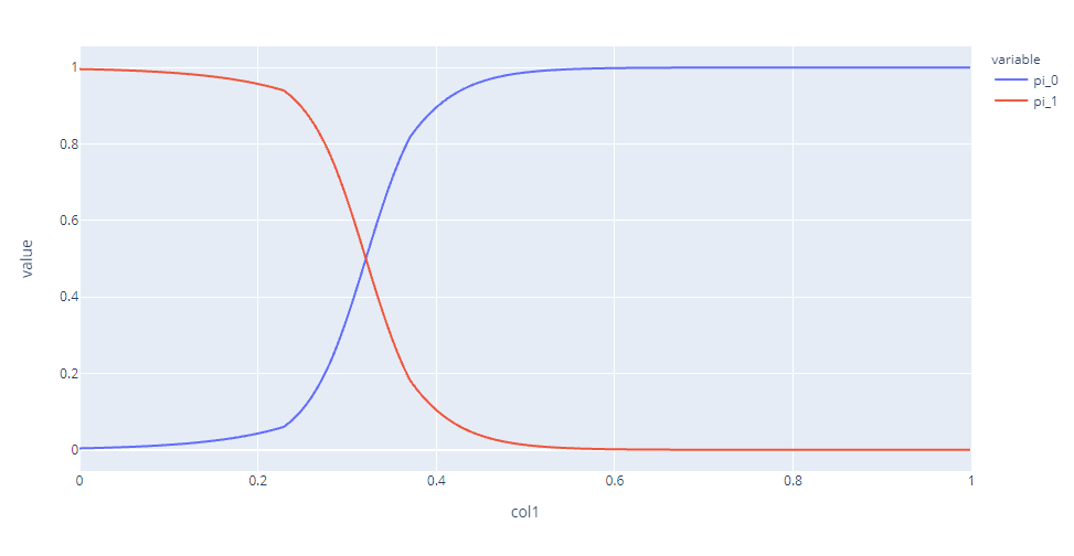
Component 1(which is the pink one in the previous plot) has high mixing coefficients till the transition point and drops to zero pretty quickly after that.

Summary

We have seen how important uncertainty is important to business decisions and also explored one way of doing that using Mixture Density networks. The implementation with all the tricks discussed in the article is available to use in a very user friendly way at PyTorch Tabular, along with a few other State of the Art algorithms for Tabular data. Check it out here:

• PyPi
• Github
• Documentation

As always for any query/questions reach out to me on LinkedIn. For any issues you face with the library, raise an issue at Github.

References

1. C. M. Bishop, Mixture density networks, (1994)
2. Vossen, Julian & Feron, Baptiste & Monti, A.. (2018). Probabilistic Forecasting of Household Electrical Load Using Artificial Neural Networks. 10.1109/PMAPS.2018.8440559.
3. Guillaumes, A.B. (2017). Mixture Density Networks for distribution and uncertainty estimation. Master Thesis. University of Barcelona
4. Jang, E., Gu, S., & Poole, B. (2017). Categorical Reparameterization with Gumbel-Softmax. ArXiv, abs/1611.01144.