The Gradient Boosters I: The Good Old Gradient Boosting

In 2001, Jerome H. Friedman wrote up a seminal paper – Greedy function approximation: A gradient boosting machine. Little did he know that was going to evolve into a class of methods which threatens Wolpert’s No Free Lunch theorem in the tabular world. Gradient Boosting and its cousins(XGBoost and LightGBM) have conquered the world by giving excellent performances in classification as well as regression problems in the realm of tabular data.

Today, I am starting a new blog series on the Gradient Boosting Machines and all its cousins. The outline for the blog series are as follows: (This will be updated with links as and when each of them gets published)

1. Part I – Gradient Boosting Algorithm
2. Part II – Regularized Greedy Forest
3. Part III – XGBoost
4. Part IV – LightGBM
5. Part V – CatBoost
6. Part VI – NGBoost
7. Part VII – The Battle of the Boosters

In the first part, let’s understand the classic Gradient Boosting methodology put forth by Friedman. Even though this is math heavy, it’s not that difficult. And wherever possible, I have tried to provide intuition to what’s happening.

Problem Setup

Let there be a dataset D with n samples. Each sample has m set of features in a vector x, and a real valued target, y. Formally, it is written as

Now, Gradient Boosting algorithms are an ensemble method which takes an additive form. The intuition is that a complex function, which we are trying to estimate, can be made up of smaller and simpler functions, added together.

Suppose the function we are trying to approximate is

We can break this function as :

This is the assumption we are taking when we choose an additive ensemble model and the Tree ensemble that we usually talk about when talking about Gradient Boosting can be written as below:

where M is the number of base learners and F is the space of regression trees.

Loss Function

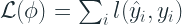
where l is the differentiable convex loss function

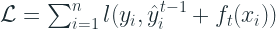
Since we are looking at an additive functional form for , we can replace with

So, the loss function will become:

Algorithm

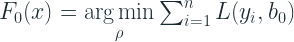
1. Initialize the model with a constant value by minimizing the loss function
   • 
   • is the prediction of the model which minimizes the loss function at 0th iteration
   • For the Squared Error loss, it works out to be the average over all training samples
   • For the Least Absolute Deviation loss, it works out to be the median over all training samples
2. for m=1 to M:
   1. Compute
      • is nothing but the derivative of the Loss Function(between true and the output from the last iteration) w.r.t. F(x) from the last iteration
      • For the Squared Error loss, this works out to be the residual(Observed – Predicted)
      • It is also called the pseudo residual because it acts like the residual and it is the residual for the Squared Error loss function
      • We calculate the for all the n samples
   2. Fit a Regression Tree to the values using Gini Impurity or Entropy (the usual way)
      • Each leaf of the tree is denoted by for , where is the number of leaves in the tree created in iteration m
   3. For compute
      • is the basis function or the least squared coefficients. This conveniently works out to be the average over all the samples in any leaf for the Squared Error loss and median for the Least Absolute Deviation loss
      • is the scaling factor or leaf weights.
      • The inner summation over can be ignored because of the disjoint nature of the Regression Trees. One particular sample will only be in one of those leaves. So the equation simplifies to:
      • 
      • So, for each of the leaves, , we calculate the optimum value , when added to the prediction of the last iteration minimizes the loss for the samples that reside in the leaf
      • For known loss functions like the Squared Error loss and Least Absolute Deviation loss, the scaling factor is 1. And because of that, the standard GBM implementation ignores the scaling factor.
      • For some losses like the Huber loss, is estimated using a line search to find the minimum loss.
   4. Update
      • Now we add the latest, optimized tree to the result from previous iteration.
      • is the shrinkage or learning rate
      • The summation in the equation is only useful in the off chance that a particular sample ends up in multiple nodes. Otherwise, it’s just the optimized regression tree score

Regularization

In the standard implementation (Sci-kit Learn), the regularization term in the objective function is not implemented. The only regularization that is implemented there are the following:

• Regularization by Shrinkage – In the additive formulation, each new weak learner is “shrunk” by a factor, . This shrinkage is also called learning rate in some implementation because it resembles the learning rate in neural networks.
• Row Subsampling – Each of the candidate trees in the ensemble uses a subset of samples. This has a regularizing effect.
• Column Subsampling – Each of the candidate trees in the ensemble uses a subset of features. This also has a regularizing effect and is usually more effective. This also helps in parallelization.

Gradient Boosting & Gradient Descent

The Similarity

We know that Gradient Boosting is an additive model and can be shows as below:

where F is the ensemble model, f is the weak learner, η is the learning rate and X is the input vector.

Substituting F with , we get the familiar equation,

Now since is obtained at each iteration by minimizing the loss function which is a function of the first and second order gradients (derivatives), we can intuitively think about that as a directional vector pointing towards the steepest descent. Let’s call this directional vector as . The subscript is m-1 because the vector has been trained on stage m-1 of the iteration. Or, intuitively the residual . So the equation now becomes:

Flipping the signs, we get:

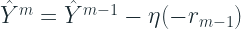
Now let’s look at the standard Gradient Descent equation:

We can clearly see the similarity. And this result is what enables us to use any differentiable loss function.

The Difference

When we train a neural network using Gradient Descent, it tries to find the optimum parameters(weights and biases), w, that minimizes the loss function. And this is done using the gradients of the loss with respect to the parameters.

But in Gradient Boosting, the gradient only adjusts the way the ensemble is created and not the parameters of the underlying base learner.

While in neural network, the gradient directly gives us the direction vector of the loss function, in Boosting, we only get the approximation of that direction vector from the weak learner. Consequently, the loss of a GBM is only likely to reduce monotonically. It is entirely possible that the loss jumps around a bit as the iterations proceed.

Implementation

GradientBoostingClassifier and GradientBoostingRegressor in Sci-kit Learn are one of the earliest implementations in the python ecosystem. It is a straight forward implementation, faithful to the original paper. I follows pretty much the discussion we had till now. And it has implemented for a variety of loss functions for which the Greedy function approximation: A gradient boosting machine[1] by Friedman had derived algorithms.

• Regression Losses
  • ‘ls’ → Least Squares
  • ‘lad’ → Least Absolute Deviation
  • ‘huber’ → Huber Loss
  • ‘quantile’ → Quantile Loss
• Classification Losses
  • ‘deviance’ → Logistic Regression loss
  • ‘exponential’ → Exponential Loss

In the next part of the series, let’s take a look at one of the lesser known cousin of Gradient Boosting – Regularized Greedy Forest

• Part I – Gradient boosting Algorithm
• Part II – Regularized Greedy Forest
• Part III – XGBoost
• Part IV – LightGBM
• Part V – CatBoost
• Part VI – NGBoost
• Part VII – The Battle of the Boosters

Stay tuned!

References

1. Friedman, Jerome H. Greedy function approximation: A gradient boosting machine. Ann. Statist. 29 (2001), no. 5, 1189–1232.