The Gradient Boosters IV: LightGBM

XGBoost reigned king for a while, both in accuracy and performance, until a contender rose to the challenge. LightGBM came out from Microsoft Research as a more efficient GBM which was the need of the hour as datasets kept growing in size. LightGBM was faster than XGBoost and in some cases gave higher accuracy as well. Although XGBoost made some changes and implemented the innovations LightGBM brought forward and caught up, LightGBM had already made it’s splash. It became a staple component in the winning ensembles in many Kaggle Competitions.

The starting point for the LightGBM was XGBoost. So essentially, they took XGBoost and optimized it, and therefore, it has all the innovations XGBoost had (more or less), and some additional ones. Let’s take a look at the incremental improvements that LightGBM made:

Leaf-wise Tree Growth

One of the main changes from all the other GBMs, like XGBoost, is the way tree is constructed. In LightGBM, a leaf-wise tree growth strategy is adopted.

All the other popular GBM implementations follow somehting called a Level-wise tree growth, where you find the best possible node to split and you split that one level down. This strategy will result in symmetric trees, where every node in a level will have child nodes resulting in an additional layer of depth.

In LightGBM, the leaf-wise tree growth finds the leaves which will reduce the loss the maximum, and split only that leaf and not bother with the rest of the leaves in the same level. This results in an asymmetrical tree where subsequent splitting can very well happen only on one side of the tree.

Leaf-wise tree growth strategy tend to achieve lower loss as compared to the level-wise growth strategy, but it also tends to overfit, especially small datasets. So small datasets, the level-wise growth acts like a regularization to restrict the complexity of the tree, where as the leaf-wise growth tends to be greedy.

Gradient-based One-Side Sampling (GOSS)

Subsampling or Downsampling is one of the ways with which we introduce variety and speed up the training process in an ensemble. It is also a form of regularization as it restricts from fitting to the complete training data. Usually, this subsampling is done by taking a random sample from the training dataset and building a tree on that subset. But what LightGBM introduced was an intelligent way of doing this downsampling.

The core of the idea is that the gradients of different samples is an indicator to how big of a role does it play in the tree building process. The instances with larger gradients (under-trained), contribute a lot more to the tree building process than instances with small gradients. So, when we downsample, we should strive to keep the instances with large gradients so that the tree building is the most efficient.

The most straightforward idea is to discard the instances with low gradients and build the tree on just the large gradient instances. But this would change the distribution of the data which in turn would hurt the accuracy of the model. And hence, the GOSS method.

The algorithm is pretty straightforward:

1. Keep all the instances with large gradients
2. Perform random sampling on instances with small gradients
3. Introduce a constant multiplier for the data instances with small gradients when computing the information gain in the tree building process.
   1. If we select a instances with large gradients and randomly samples b instances with small gradients, we amplify the sampled data by

Exclusive Feature Bundling (EFB)

The motivation behind EFB is a common theme between LightGBM and XGBoost. In many real world problems, although there are a lot of features, most of them are really sparse, like on-hot encoded categorical variables. The way LightGBM tackles this problem is slightly different.

The crux of the idea lies in the fact that many of these sparse features are exclusive, i.e. they do not take non-zero values simultaneously. And we can efficiently bundle these features and treat them as one. But finding the optimal feature bundles is an NP-Hard problem.

To this end, the paper proposes a Greedy Approximation to the problem, which is the Exclusive Feature Bundling algorithm. The algorithm is also slightly fuzzy in nature, as it will allow bundling features which are not 100% mutually exclusive, but it tries to maintain the balance between accuracy and efficiency when selecting the bundles.

The algorithm, on a high level, is:

1. Construct a graph with all the features, weighted by the edges which represents the total conflicts between the features
2. Sort the features by their degrees in the graph in descending order
3. Check each feature and either assign it to an existing bundle with a small conflict or create a new bundle.

Histogram-based Tree Splitting

The amount of time it takes to build a tree is proportional to the number of splits that have to be evaluated. And when you have continuous or categorical features with high cardinality, this time increases drastically. But most of the splits that can be made for a feature only offer miniscule changes in performance. And this concept is why a histogram based method is applied to tree building.

The core idea is to group features into set of bins and perform splits based on these bins. This reduces the time complexity from O(#data) to O(#bins).

Sparse Inputs

In another innovation, similar to XGBoost, LightGBM ignores the zero feature values while creating the histograms. And this reduces the cost of building the histogram from O(#data) to O(#non-zero data).

Categorical Features

In many real world datasets, Categorical features make a big presence and thereby it becomes essential to deal with them appropriately. The most common approach is to represent a categorical feature as it’s one-hot representation, but this is sub-optimal for tree learners. If you have high-cardinality categorical features, your tree needs to be very deep to achieve accuracy.

LightGBM takes in a list of categorical features as an input so that it can deal with it more optimally. It takes inspiration from “On Grouping for Maximum Homogeneity” by Fisher, Walter D. and uses the following methodology for finding the best split for categorical features.

1. Sort the histogram on accumulated gradient statistics
2. Find the best split on the sorted histogram

There are a few hyperparameters which help you tune the way the categorical features are dealt with[4]:

• cat_l2 , default = 10.0, type = double, constraints: cat_l2 >= 0.0
  • used for the categorical features
  • L2 regularization in categorical split
• cat_smooth , default = 10.0, type = double, constraints: cat_smooth >= 0.0
  • used for the categorical features
  • this can reduce the effect of noises in categorical features, especially for categories with few data
  • max_cat_to_onehot , default = 4, type = int, constraints: max_cat_to_onehot > 0
    • when number of categories of one feature smaller than or equal to max_cat_to_onehot, one-vs-other split algorithm will be used

Performance Improvements

The majority of the incremental performance improvements were made through GOSS and EFB.

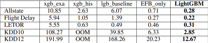
xgb_exa is the original XGBoost, xgb_his is the histogram based version(which came out later), lgb_baseline is the LightGBM without EFB and GOSS, and LightGBM is with EFB and GOSS. It is quite evident that the improvement in GOSS and EFB is phenomenal as compared to lgb_baseline.

The rest of the improvements in performance is derived from the ability to parallelize the learning. There are two main ways of parallelizing the learning process:

Feature Parallel

Feature Parallel tries to parallelize the “Find the best split” part in a distributed manner. Evaluating different splits are done in parallel across multiple workers, and then they communicate with each other to decide among themselves who has the best split.

Data Parallel

Data Parallel tries to parallelize the whole decision learning. In this, we typically split the data and send different parts of the data to different workers who calculate the histograms based on the section of the data they receive. Then they communicate to merge the histogram at a global level and this global level histogram is what is used in the tree learning process.

Voting Parallel

Voting Parallel is a special case of Data Parallel, where the communication cost in Data Parallel is capped to a constant.

HyperParameters

LightGBM is one of those algorithms which has a lot, and I mean a lot, of hyperparameters. It is so flexible that it is intimidating for the beginner. But there is a way to use the algorithm and still not tune like 80% of those parameters. Let’s look at a few parameters that you can start tuning and then build up confidence and start tweaking the rest.

• objective 🔗︎, default = regression, type = enum, options: regression, regression_l1, huber, fair, poisson, quantile, mape, gamma, tweedie, binary, multiclass, multiclassova, cross_entropy, cross_entropy_lambda, lambdarank, rank_xendcg, aliases: objective_type, app, application
• boosting 🔗︎, default = gbdt, type = enum, options: gbdt, rf, dart, goss, aliases: boosting_type, boost
  • gbdt, traditional Gradient Boosting Decision Tree, aliases: gbrt
  • rf, Random Forest, aliases: random_forest
  • dart, Dropouts meet Multiple Additive Regression Trees
  • goss, Gradient-based One-Side Sampling
• learning_rate 🔗︎, default = 0.1, type = double, aliases: shrinkage_rate, eta, constraints: learning_rate > 0.0
  • shrinkage rate
  • in dart, it also affects on normalization weights of dropped trees
• num_leaves 🔗︎, default = 31, type = int, aliases: num_leaf, max_leaves, max_leaf, constraints: 1 < num_leaves <= 131072
  • max number of leaves in one tree
• max_depth 🔗︎, default = -1, type = int
  • limit the max depth for tree model. This is used to deal with over-fitting when #data is small. Tree still grows leaf-wise
  • <= 0 means no limit
• min_data_in_leaf 🔗︎, default = 20, type = int, aliases: min_data_per_leaf, min_data, min_child_samples, constraints: min_data_in_leaf >= 0
  • minimal number of data in one leaf. Can be used to deal with over-fitting
• min_sum_hessian_in_leaf 🔗︎, default = 1e-3, type = double, aliases: min_sum_hessian_per_leaf, min_sum_hessian, min_hessian, min_child_weight, constraints: min_sum_hessian_in_leaf >= 0.0
  • minimal sum hessian in one leaf. Like min_data_in_leaf, it can be used to deal with over-fitting
• lambda_l1 🔗︎, default = 0.0, type = double, aliases: reg_alpha, constraints: lambda_l1 >= 0.0
  • L1 regularization
• lambda_l2 🔗︎, default = 0.0, type = double, aliases: reg_lambda, lambda, constraints: lambda_l2 >= 0.0
  • L2 regularization

In the next part of our series, let’s look at the one who tread a path less taken – CatBoost

• Part I – Gradient boosting Algorithm

• Part I – Gradient boosting Algorithm
• Part II – Regularized Greedy Forest
• Part III – XGBoost
• Part IV – LightGBM
• Part V – CatBoost
• Part VI(A) – Natural Gradient
• Part VI(B) – NGBoost
• Part VII – The Battle of the Boosters

References

1. Friedman, Jerome H. Greedy function approximation: A gradient boosting machine. Ann. Statist. 29 (2001), no. 5, 1189–1232.
2. Ke, Guolin et.al. (2017). LightGBM: A Highly Efficient Gradient Boosting Decision Tree. In Advances in Neural Information Processing Systems, pages 3149-3157
3. Walter D. Fisher. “On Grouping for Maximum Homogeneity.” Journal of the American Statistical Association. Vol. 53, No. 284 (Dec., 1958), pp. 789-798.
4. LightGBM Parameters. https://github.com/microsoft/LightGBM/blob/master/docs/Parameters.rst#core-parameters