The Gradient Boosters VI(B): NGBoost

The reign of the Gradient Boosters were almost complete in the land of tabular data. In most real world as well as competitions, there was hardly a solution which did not have at least one model from one of the gradient boosting algorithms. But as the machine learning community matured, and the machine learning applications started to be more in use, the need for uncertainty output became important. For classification, the output from Gradient Boosting was already in a form which lets you understand the confidence of the model in its prediction. But for regression problems, it wasn’t the case. The model spat out a number and told us this was its prediction. How do you get uncertainty estimates from a point prediction? And this problem was not just for Gradient Boosting algorithms. but was for almost all the major ML algorithms. This is the problem that the new kid on the block – NGBoost seeks to tackle.

If you’ve not read the previous parts of the series, I strongly advise you to read up, at least the first one where I talk about the Gradient Boosting algorithm, because I am going to take it as a given that you already know what Gradient Boosting is. I would also strongly suggest to read the VI(A) so that you have a better understanding of what Natural Gradients are

Natural Gradient Boosting

The key innovation in NGBoost is the use of Natural Gradients instead of regular gradients in the boosting algorithm. And by adopting this probabilistic route, it models a full probability distribution over the outcome space, conditioned on the covariates.

The paper modularizes their approach into three components –

Base Learner
Parametric Distribution
Scoring Rule

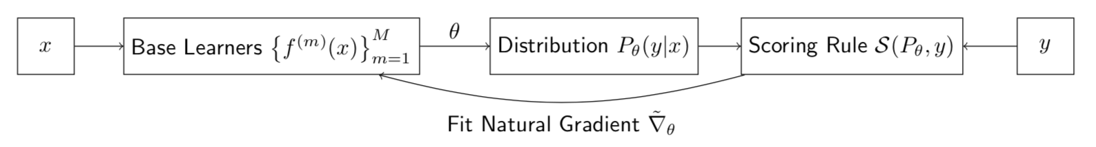
Base Learners

As in any boosting technique, there are base learners which are combined together to get a complete model. And the NGBoost doesn’t make any assumptions and states that the base learners can be any simple model. The implementation supports a Decision Tree and ridge Regression as base learners out of the box. But you can replace them with any other sci-kit learn style models just as easily.

Parametric Distribution

Here, we are not training a model to predict the outcome as a point estimate, instead we are predicting a full probability distribution. And every distribution is parametrized by a few parameters. For eg., the normal distribution is parametrized by its mean and standard deviation. You don’t need anything else to define a normal distribution. So, if we train the model to predict these parameters, instead of the point estimate, we will have a full probability distribution as the prediction.

Scoring Rule

Any machine learning system works on a learning objective, and more often than not, it is the task of minimizing some loss. In point prediction, the predictions are compared with data with a loss function. Scoring rule is the analogue from the probabilistic regression world. The scoring rule compares the estimated probability distribution with the observed data.

A proper scoring rule, $\mathcal{S}$ , takes as input a forecasted probability distribution $\mathcal{P}$ and one observation $y$ (outcome), and assigns a score $\mathcal{S}(\mathcal{P},y)$ to the forecast such that the true distribution of the outcomes gets the best score in expectation.

The most commonly used proper scoring rule is the logarithmic score $\mathcal{L}$ , which, when minimized we get the MLE

$\mathcal{L}(\theta,y) = -log \mathcal{P}_{\theta}(y)$

which is nothing but the log likelihood that we have seen in so many places. And the scoring rule is parametrized by $\theta$ because that is what we are predicting as part of the machine learning model.

Another example is CRPS(Continuous Ranked Probability Score). While the logarithmic score or the log likelihood generalizes Mean Squared Error to a probabilistic space, CRPS does the same to Mean Absolute Error.

$\mathcal{C}(\theta, y) = \int_{-\infty}^{y} F_{\theta}(z)^2 dz + \int_{y}^{\infty} (1- F_{\theta}(z))^2dz$

Generalized Natural Gradient

In the last part of the series, we saw what Natural Gradient was. And in that discussion, we talked abut KL Divergences, because traditionally, Natural Gradients were defined on the MLE scoring rule. But the paper proposes a generalization of the concept and provide a way to extend the concept to CRPS scoring rule as well. They generalized KL Divergence to a general Divergence and provided derivations for CRPS scoring rule.

Putting it all together

Now that we have seen the major components, let’s take a look at how all of this works together. NGBoost is a supervised learning method for probabilistic prediction that uses boosting to estimate the parameters of a conditional probability distribution $\mathcal{P}(y|x)$ . As we saw earlier, we need to choose three modular components upfront:

Base learner ( $f$ )
Parametric Probability Distribution ( $\mathcal{P}_{\theta}$ )
Proper scoring rule ( $\mathcal{S}$ )

A prediction $y|x$ on a new input x is made in the form of a conditional distribution $\mathcal{P}_{\theta}$ , whose parameters $\theta$ are obtained by an additive combination of M base learners outputs and in initial $\theta_0$ . Let’s denote the combined function learned by the M base learners for all parameters by $f^{(m)}$ . And there will be a separate set of base learners for each parameter in the chosen probability distribution. For eg. in the normal distribution, there will be $f_{\mu}^{(m)}$ and $f_{log \sigma}^{(m)}$ .

The predicted outputs are also scaled with a stage specific scaling factor ( $\rho^{(m)}$ ), and a common learning rate $\eta$ :

$y|x \sim \mathcal{P}{\theta}(x), \theta = \theta_0+\eta\sum_{m=1}^{M}\rho^{(m)} \cdot f^{(m)}(x)$

One thing to note here is that even if you have n parameters for your probability distribution, $\rho$ is still a single scalar.

Algorithm

Let us consider a Dataset $\mathcal{D} = {x_i, y_i}_{i=1}^{n}$ , Boosting Iterations M, Learning rate $\eta$ , Probability Distribution with parameters $\theta$ , Proper scoring rule $\mathcal{S}$ , and Base learner $f$

Initialize $\theta_0$ to the marginal. This is just estimating the parameters of the distribution without conditioning on any covariates; similar to initializing to mean. Mathematically, we solve this equation:
$arg min_{\theta} \sum_{i=1}^{n} S(\theta,y_i)$
For each iteration in M:
1. Calculate the Natural gradients $g_i^{(m)}$ of the Scoring rule S with respect to the parameters at previous stage $\theta_i^{(m-1)}$ for all n examples in dataset.
2. A set of base learners for that iteration $f^{(m)}$ are fit to predict the corresponding components of the natural gradients, $g_i^{(m)}$ . This output can be thought of as the projection of the natural gradient on to the range of the base learner class, because we are training the base learners to predict the natural gradient at current stage.
3. This projected gradient is then scaled by a scaling factor $\rho^{(m)}$ . This is because Natural Gradients rely on local approximations(as we saw in the earlier post) and these local approximations won’t hold good far away from the current parameter position.
  In practice, we use a line search to get the best scaling factor which minimizes the overall scoring rule. In the implementation, they have found out that reducing the scaling factor by half in the line search works well.
4. Once the scaling parameter is estimated, we update the parameters by adding the negative scaled projected gradient to the outputs of previous stage, after further scaling by a learning rate.
  $\theta_i^{(m)} \leftarrow \theta_i^{(m-1)} - \eta(\rho^{(m)} \cdot f^{(m)}(x_i))$

Implementation

The algorithm has a ready use Sci-kit Learn style implementation at https://github.com/stanfordmlgroup/ngboost. Let’s take a look at the key parameters to tune in the model.

Hyperparameters

Dist : This parameter sets the distribution of the output. Currently, the library supports Normal, LogNormal, and Exponential distributions for regression, k_categorical and Bernoulli for classification. Default: Normal
Score : This specifies the scoring rule. Currently the options are between LogScore or CRPScore. Default: LogScore
Base: This specifies the base learner. This can be any Sci-kit Learn estimator. Default is a 3-depth Decision Tree
n_estimators : The number of boosting iterations. Default: 500
learning_rate: The learning rate. Default:0.01
minibatch_frac : The percent subsample of rows to use in each boosting iteration. This is more of a performance hack than performance tuning. When the data set is huge, this parameter can considerably speed things up.

Interpretation

Although there needs to be a considerable amount of caution before using the importances from machine learning models, NGBoost also offers feature importances. It has separate set of importances for each parameter it estimates.

But the best part is not just this, but that SHAP, is also readily available for the model. You just need to use TreeExplainer to get the values.(To know more about SHAP and other interpretable techniques, check out my other blog series – Interpretability: Cracking open the black box).

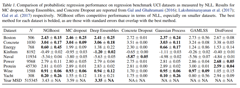
Experiments

The paper also looks at how the algorithm performs when compared to other popular algorithms. There were two separate type of evaluation – Probabilistic, and Point Estimation

Probabilistic Regression

On a variety of datasets from the UCI Machine Learning Repository, NGBoost was compared with other major probabilistic regression algorithms, like Monte-Carlo Dropout, Deep Ensembles, Concrete Dropout, Gaussian Process, Generalized Additive Model for Location, Scale and Shape(GAMLSS), Distributional Forests.

Point Estimate

They also evaluated the algorithm on the point estimate use case against other regression algorithms like, Elastic Net, Random Forest(Sci-kit Learn), Gradient Boosting(Sci-kit Learn).

Conclusions

NGBoost performs as well or better than the existing algorithms, but also has an additional advantage of providing us a probabilistic forecast. And the formulation and implementation are flexible and modular enough to make it easy to use.

But one drawback here is with the performance of the algorithm. The time complexity linearly increases with each additional parameter we have to estimate. And all the efficiency hacks/changes which has made its way into popular Gradient Boosting packages like LightGBM, or XGBoost are not present in the current implementation. Maybe it would be ported over soon enough because I see the repo is under active development and see this as one of the action items they are targeting. But until that happens, this is quite slow, especially with large data. One way out is to use minibatch_frac parameter to make the calculation of natural gradients faster.

Now that we have seen all the major Gradient Boosters, let’s pick a sample dataset and see how these performs in the next part of the series.

Part I – Gradient boosting Algorithm
Part II – Regularized Greedy Forest
Part III – XGBoost
Part IV – LightGBM
Part V – CatBoost
Part VI(A) – Natural Gradient
Part VI(B) – NGBoost
Part VII – The Battle of the Boosters

References

Amari, Shun-ichi. Natural Gradient Works Efficiently in Learning. Neural Computation, Volume 10, Issue 2, p.251-276.
Duan, Tony. NGBoost: Natural Gradient Boosting for Probabilistic Prediction, arXiv:1910.03225v4 [cs.LG] 9 Jun 2020
NGBoost documentation, https://stanfordmlgroup.github.io/ngboost

4 thoughts on “The Gradient Boosters VI(B): NGBoost”

Pingback: The Gradient Boosters V: CatBoost – Deep & Shallow
Pingback: The Gradient Boosters IV: LightGBM – Deep & Shallow
Pingback: The Gradient Boosters VII: Battle of the Boosters – Deep & Shallow
Pingback: PyTorch Tabular – A Framework for Deep Learning for Tabular Data – Deep & Shallow

The Gradient Boosters VI(B): NGBoost