The Gradient Boosters III: XGBoost

Now let’s get the elephant out of the way – XGBoost. This is the most popular cousin in the Gradient Boosting Family. XGBoost with its blazing fast implementation stormed into the scene and almost unanimously turned the tables in its favor. Soon enough, Gradient Boosting, via XGBoost, was the reigning king in Kaggle Competitions and pretty soon, it trickled down to the business world.

There were a few key innovations that made XGBoost so effective:

Explicit Regularization

Similar to Regularized Greedy Forest, XGBoost also has an explicit regularization term in the objective function.

is the regularization term which penalizes T, the number of leaves in the tree and is the regularization term which penalizes w, the weights of different leaves.

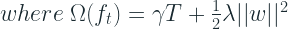
This is a much simpler regularization term than some of the ways we saw in Regularized Greedy Forest.

Objective Function Agnostic Implementation

One of the key ingredients of Gradient Boosting algorithms is the gradients or derivatives of the objective function. And all the implementations that we saw earlier used pre-calculated gradient formulae for specific loss functions, thereby, restricting the objectives which can be used in the algorithm to a set which is already implemented in the library.

XGBoost uses the Newton-Raphson method we discussed in a previous part of the series to approximate the loss function.

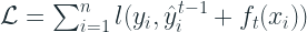
Now, the complex recursive function made up of tree structures can be approximated using Taylor’s approximation into a differentiable form. In the case of Gradient Boosting, we take the second order approximation, meaning we use two terms – first order derivative and second order derivative- to approximate the function.

Let,

Approximated Loss function:

The first term, the loss, is constant at a tree building stage, t, and because of that it doesn’t add any value to the optimization objective. So removing it and simplifying we get,

Substituting the Ω with the regularization term, we get:

The f(x) we are talking about is essentially a tree with leaf weights, w. So if we define as the instance set in leaf j, we can substitute the tree structure directly into the equation and simplify as:

Setting this equation to zero we can find the optimum value for as :

Putting this back into the loss function and simplifying we get:

What all of this enables us to do is to separate out the objective function from the core working of the algorithm. And by adopting this formulation, the only requirement from an objective function/loss function is that it needs to be differentiable. To be very specific, the loss function should return the first and second order derivatives.

See here for a list of all the objective functions that are pre-built into XGBoost.

Tree Building Strategy

The tree building strategy lies somewhat in between classical Gradient Boosting and regularized Greedy Forests. While the classical Gradient Boosting takes the tree at each stage as a black box, Regularized Greedy Forest operates at a leaf level by updating any part of the forest at each step. XGBoost takes a middle ground and considers a tree that is made in a previous iteration sacrosanct, but while making a tree for any iteration, it doesn’t use the standard impurity measures, but the gradient based Loss function we derived in the last section in the tree building process. While in classic Gradient Boosting the optimization of the loss function happens after the tree is built, XGBoost gets that optimization during the tree building process as well.

Normally its impossible to enumerate all possible tree structures. Therefore a greedy algorithm is implemented that starts from a single leaf and iteratively adds branches to the tree based on the simplified loss function

Split-finding Algorithm

One of the key problems in tree learning is to find the best split. Usually, we will have to enumerate all the possible splits over all the features and then use the impurity criteria to choose the best split. This is called exact greedy algorithm. It is computationally demanding, especially for continuous and high cardinality categorical features. And it also not feasible when the data doesn’t fit into memory.

To overcome these inefficiencies, the paper proposes an Approximate Algorithm. It first proposes candidate splitting points according to the percentiles of the features. On a highlevel, the algorithm is:

1. Propose candidate splitting points for all the features using the percentiles of the features
2. Map the continuous features to buckets split by the candidate splitting points
3. Aggregate the gradient statistics for all the features based on the candidate splitting points
4. Finds the best solution among proposals based on aggregate statistics

Weighted Quantile Sketch

One of the important steps in the algorithm discussed above is the proposal of candidate splits. usually percentiles of a feature are used to make candidates distribute evenly on the data. And a set of algorithms which does that in a distributed manner and with speed and efficiency are called Quantile sketching algorithms. But here, the problem is slightly complicated because the need is to have a weighted quantile sketching algorithm which weighs the instances based on the gradient(so that we can learn the most from instances with most error). So they proposed a new data structure which has provable theoretical guarantee.

Sparsity-aware Split Finding

This is another key innovation in XGBoost and this came from the realization that real-world datasets are sparse. This sparsity can come form multiple causes,

1. Presence of missing values in the data
2. Frequent zero values
3. Artifacts of feaature engineering such as One-Hot Encoding

And for this reason, the authors decide to make the algorithm aware of the sparsity so that it can be dealt with intelligently. And the way they made that is deceivingly simple.

They gave a default direction in each tree node. i.e. if a value is missing or zero, that instance flows down a default direction in the branch. And the optimal default direction is learned from the data

This innovation has a two fold benefit –

1. it helps group the missing values learn an optimal way of handling them
2. it boosts the performance by making sure no computing power is wasted in trying to find gradient statistics for missing values.

Performance Improvements

One of the main drawbacks of all the implementations of the Gradient Boosting algorithm were that they were quite slow. While the forest creation in a Random Forest was parallel out of the box, Gradient Boosting was a sequential process which builds new base learners on old ones. One of XGBoost’s claim to fame was how blazingly fast it was. It was at least 10 times faster than the existing implementations and it was able to work with large datasets because of the out-of-core learning capabilities. The key innovations in performance improvement were:

Column Block for Parallel Learning

The most time consuming part of tree learning is to get the data sorted into order. The authors of the paper proposed to store the data in in-memory units, called blocks. Data in each block is sorted in the Compressed column (CSC) format. This input data layout is computed once before training and reused thereafter. By handing the data in this sorted format, the tree split algorithm is reduced to a linear scan over the sorted columns

Cache-aware Access

While the proposed block structure helps optimize the computation complexity of split finding, it requires indirect fetches of gradient statistics by row index. To get over the slow write and read operations in the process, the authors implemented an internal buffer for each thread and accumulate the gradient statistics in minibatches. This helps in reducing the runtime overhead when the rows are large.

Blocks for Out-of-core Computation

One of the goals of the algorithm is to fully utilize the machine’s resources. While the CPUs are utilized by parallelization of the process, the available disk space is utilized by the out-of-core learning. These blocks that we saw earlier are stored on disk and a separate prefetch thread keeps fetching the data into memory just in time for the computation to continue. They use two techniques to make the I/O operations from disk faster –

• Block Compression, where each block is compressed before storage and uncompressed on the fly while reading.
• Block Sharding, where a block is broken down into multiple pieces and stored across multiple disks(if any). And the prefetcher reads the block by alternating between the two disks, thereby increasing throughput of the disk reading.

HyperParameters

XGBoost has so many articles and blogs about it covering the hyperparameters and how to tune them that I’m not even going to attempt it.

The single source of truth for any hyperparameter is the official documentation. It might be intimidating to look at the long list of hyperparameters there, but you won’t end up touching the majority of them in a normal use case.

The major ones are:

• eta [default=0.3, alias: learning_rate]
  • Step size shrinkage used in update to prevents overfitting. After each boosting step, we can directly get the weights of new features, and eta shrinks the feature weights to make the boosting process more conservative.
  • range: [0,1]
• gamma [default=0, alias: min_split_loss]
  • Minimum loss reduction required to make a further partition on a leaf node of the tree. The larger gamma is, the more conservative the algorithm will be.
  • range: [0,∞]
• max_depth [default=6]
  • Maximum depth of a tree. Increasing this value will make the model more complex and more likely to overfit. 0 is only accepted in lossguided growing policy when tree_method is set as hist and it indicates no limit on depth. Beware that XGBoost aggressively consumes memory when training a deep tree.
  • range: [0,∞] (0 is only accepted in lossguided growing policy when tree_method is set as hist)
• min_child_weight [default=1]
  • Minimum sum of instance weight (hessian) needed in a child. If the tree partition step results in a leaf node with the sum of instance weight less than min_child_weight, then the building process will give up further partitioning. In linear regression task, this simply corresponds to minimum number of instances needed to be in each node. The larger min_child_weight is, the more conservative the algorithm will be.
  • range: [0,∞]
• subsample [default=1]
  • Subsample ratio of the training instances. Setting it to 0.5 means that XGBoost would randomly sample half of the training data prior to growing trees. and this will prevent overfitting. Subsampling will occur once in every boosting iteration.
  • range: (0,1]
• colsample_bytree, colsample_bylevel, colsample_bynode [default=1]
  • This is a family of parameters for subsampling of columns.
  • All colsample_by* parameters have a range of (0, 1], the default value of 1, and specify the fraction of columns to be subsampled.
  • colsample_bytree is the subsample ratio of columns when constructing each tree. Subsampling occurs once for every tree constructed.
  • colsample_bylevel is the subsample ratio of columns for each level. Subsampling occurs once for every new depth level reached in a tree. Columns are subsampled from the set of columns chosen for the current tree.
  • colsample_bynode is the subsample ratio of columns for each node (split). Subsampling occurs once every time a new split is evaluated. Columns are subsampled from the set of columns chosen for the current level.
  • colsample_by* parameters work cumulatively. For instance, the combination {‘colsample_bytree’:0.5, ‘colsample_bylevel’:0.5, ‘colsample_bynode’:0.5} with 64 features will leave 8 features to choose from at each split.
• lambda [default=1, alias: reg_lambda]
  • L2 regularization term on weights. Increasing this value will make model more conservative.
• alpha [default=0, alias: reg_alpha]
  • L1 regularization term on weights. Increasing this value will make model more conservative.

update – 13-02-2020

Leaf-wise Tree Growth

After publishing this, I came to realize I haven’t talked about some of the later developments in XGBoost like leaf-wise tree growth and how tuning the parameters are slightly different for the new faster implementation.

LightGBM, about which we will be talking about in the next blog in the series, implemented leaf-wise tree growth and that led to a huge performance improvement. XGBoost also played catch-up and implemented the leaf-wise strategy in a histogram based tree splitting strategy.

Leaf-wise growth policy, while faster, also overfits faster if the data is small. Therefore it is quite important to use regularization or cap tree complexity through hyperparameters. But if we just keep tuning max_depth as before to control complexity, it won’t work. num_leaves (which controls the number of leaves in a tree) also need to be tuned together. This is because with the same depth, a leaf-wise tree growing algorithm can make a more complex tree.

You can enable leaf-wise tree building in XGBoost by setting tree_method parameter to “hist” and the grow_policy parameter to “lossguide”

In the next part of our series, let’s look at the one who challenged the king – LightGBM

• Part I – Gradient boosting Algorithm
• Part II – Regularized Greedy Forest
• Part III – XGBoost
• Part IV – LightGBM
• Part V – CatBoost
• Part VI – NGBoost
• Part VII – The Battle of the Boosters

References

1. Friedman, Jerome H. Greedy function approximation: A gradient boosting machine. Ann. Statist. 29 (2001), no. 5, 1189–1232.
2. Chen, Tianqi & Guestrin, Carlos. (2016). XGBoost: A Scalable Tree Boosting System. 785-794. 10.1145/2939672.2939785.