The Gradient Boosters II: Regularized Greedy Forest

In 2011, Rie Johnson and Tong Zhang, proposed a modification to the Gradient Boosting model. they called it Regularized Greedy Forest. When they came up with the modification, GBDTs were already, sort of, ruling the tabular world. They tested the new modification of a wide variety of datasets, both synthetic and real world, and found that their modification achieves a better performance than standard GBDTs. They also entered a few Kaggle type competitions (Bond Price challenge, Biological Response Prediction, and Heritage Provider Network Health Prize) and won them beating out other GBDT models in the running.

The implementation(both the original and a faster multi-core version) is on the Github Page : https://github.com/RGF-team/rgf

The key modifications to the core GBDT algorithm they suggested are as follows:

Fully Corrective Greedy Update

According to Friedman[1], one of the disadvantages of the standard Gradient Boosting is that the shrinkage/learning rate, needs to be small to achieve convergence. In fact, he argued for infinitesimal step size. They suggested a modification which made the shrinkage parameter unnecessary.

In standard Gradient Boosting, the algorithm does a partial corrective step in each iteration. The algorithm only optimizes the base learner in the current iteration and ignores all the previous ones. It creates the best regression tree for the current timestep and adds it to the ensemble. But they proposed that at every iteration, we update the whole forest(m base learners for iteration m) and readjust the scaling factor at each iteration.

Structured Sparsity Regularization

While the fully corrective greedy update means that the algorithm will converge faster, it also means that it overfitted faster. Therefore Structured Sparsity Regularization was adopted to combat this problem. The general idea of structured sparsity is that in a situation where a sparse solution is assumed, one can take advantage of the sparsity structure underlying the task. In this specific setting, it was implemented as a sparse search of decision rules in the forest structure.

Explicit Regularization

In addition to the Structured Sparsity Regularization, they also included an explicit Regularization term to the loss function.

where l is the differentiable convex loss function and Ω is the regularisation term penalising the complexity of the tree structure, and is the Forest structure.

The paper introduces three types of Regularization options:

L2 Regularization on Leaves

where is the forest structure, is the constant for controlling the strength of regularization, are the weights of the node v (which is restricted to leaf nodes), is the leaves of the tree T, and is the set of all Trees in the forest.

hyperparameter in implementation: l2

Minimum-penalty Regularization

The minimum penalty regularization penalises the depth of the trees. This is a regularization that acts on all nodes and not just the leaves of the trees. This uses the principle that any leaf node can be written in terms of its ancestor nodes. The intuition behind the regularization is that it penalises depth, which is conceptually a complex decision rule.

The exact formula is beyond our scope, but the key hyperparameters in there are l2 which governs the overall strength of regularization, and reg_depth which controls how severely you penalise the depth of a tree. Suggested values for l2 are 1, 0.1, 0.01 and reg_depth should be a value greater than 1

Minimum-penalty Regularization with Sum-to-Zero Siblings

This is very similar to Minimum-penalty regularization, but with an added condition that the weights of sibling nodes should sum to zero. The intuition behind the sum-to-zero constraint is that less redundant models are preferable and that the models are least redundant when branches at internal nodes lead to completely opposite actions, like adding ‘x’ to versus subtracting ‘x’ from the output value. So this penalises two things- depth of the tree and redundancy of the tree. There are no additional hyperparameters here.

Note: An interesting tidbit to note here is that all the bechmarks in the paper and the competitions only used simple L2 regularization.

Algorithm

The general concept is still similar to Gradient Boosting, but the key differences are in the tree updates in each iteration. And also the easy and convenient derivations or gradients to be mean or median does not work anymore because of the regularization term in the objective function.

Let’s look at the new algorithm, albeit at a high level.

1. repeat
   1. is the optimum forest that minimizes among all the forests that can be obtained by applying one step of structure-changing operation to the current forest
   2. Optimize the leaf weights in to minimize the loss
2. until some exit criteria is met
3. Optimize the leaf weights in to minimize the loss
4. return

Tree building Strategy

There is one key difference in the way the trees are built in the forest in Regularized Greedy Forest. In classical Gradient Boosting, at each stage a new tree is built, with a specific criteria of stopping, like depth or number of leaves. Once you pass a stage, you do not touch that tree or the weights associated with it. On the contrary, in RGF, at any m iteration, the option to update any of the previously created m-1 trees or starting a new tree is open. The exact update to the forest is determined by the action which minimizes the loss function.

Let’s look at an example to understand the fundamental difference in Tree Building between Gradient Boosting and Regularized Greedy Forest

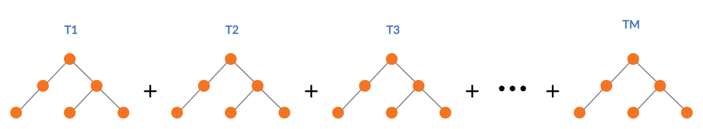
Standard Gradient Boosting builds successive trees and sum those up into an additive function which approximates the desired function.

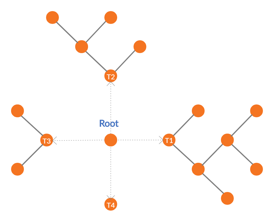
RGF takes a slightly different route. For each step change in the structure of the tree, it evaluates the possibility of growing a new leaf in an existing tree vs starting a new tree with the help of the loss function, and then takes the greedy approach of taking the route with least loss. So in the diagram above, we can choose to grow leaves in T1, T2, or T3, or we can start a new tree T4 depending on which one gives you the most reduction in loss.

But practically, it is computationally challenging to do this as the possible splits to evaluate grows exponentially as we move deeper and deeper into the forest. So, there is a hyperparameter, n_tree_search, in the implementation which restricts the retrospective update of trees to those many latest trees only. The default value is set as 1 so that the update always looks at one previously created tree. In our example, this reduces the possibilities to growing leaves in T3 or growing a new tree T4.

Conceptually, this becomes an additive function over leaves of the forest than an additive function of trees in a forest, and consequently, there is not max_depth parameter in RGF as the depth of the tree is automatically restrained by the incremental updates to the tree structure.

The next step is the weights of the new leaf that was selected to be the best structural change. This is an optimization problem and can be solved using any of the multiple methods like Gradient Descent, or Newton-Raphson’s method. Since the optimization that we are looking at is simpler, the paper uses a Newton’s step, which is much more accurate than Gradient Descent, to get an approximately optimal weight for the new leaf. Refer to Appendix A, if you are interested in how and why we need a Newton’s step to optimize such functions.

Weight Optimization

With the base learner or the basis function fixed, we need to optimize the weights of all the leaves in the forest. This is again an optimization problem, and this is solved using Cordinate Descent, which iteratively go through each of the leaves and update the weights by a Newton Step with a small step size.

Since the initial weights that is already set are approximately optimal, we do not need to re-optimize the weights every iteration. It would be computationally expensive if we do that. This is another hyperparameter in the implementation called opt_interval. Empirically, it was observed that unless opt_interval is an extreme value, the choice of opt_interval is not critical. For all the competitions they won, they had simply set the value as 100.

Key Hyperparameters and Tuning

Below is a list of key Hyperparameters that the authors of the paper suggest. It is almost directly taken from their Github Page, but adopted to the Python Wrapper.

Parameters to control training
algorithm=	RGF | RGF_Opt | RGF_Sib (Default: RGF)RGF: RGF with  regularization on leaf-only models.RGF_Opt: RGF with min-penalty regularization.RGF_Sib: RGF with min-penalty regularization with the sum-to-zero sibling constraints.
loss=	Loss function . LS | Expo | Log (Default: LS)LS: square loss .Expo: exponential loss .Log: logistic loss .
max_leaf=	Training will be terminated when the number of leaf nodes in the forest reaches this value. It should be large enough so that a good model can be obtained at some point of training, whereas a smaller value makes training time shorter. Appropriate values are data-dependent and in [2] varied from 1000 to 10000. (Default: 10000)
normalize	If turned on, training targets are normalized so that the average becomes zero. It was turned on in all the regression experiments in [2].
l2=	. Used to control the degree of  regularization. Crucial for good performance. Appropriate values are data-dependent. Either 1.0, 0.1, or 0.01 often produces good results though with exponential loss (loss=Expo) and logistic loss (loss=Log) some data requires smaller values such as 1e-10 or 1e-20.
sl2=	. Override  regularization parameter  for the process of growing the forest. That is, if specified, the weight correction process uses  and the forest growing process uses . If omitted, no override takes place and  is used throughout training. On some data,  works well.
reg_depth=	Must be no smaller than 1. Meant for being used with algorithm=RGF_Opt|RGF_Sib. A larger value penalizes deeper nodes more severely. (Default: 1)
test_interval=	Test interval in terms of the number of leaf nodes. For example, if test_interval=500, every time 500 leaf nodes are newly added to the forest, end of training is simulated and the model is tested or saved for later testing. For efficiency, it must be either multiple or divisor of the optimization interval (opt_interval: default 100). If not, it may be changed by the system automatically. (Default: 500)
n_tree_search=	Number of trees to be searched for the nodes to split. The most recently-grown trees are searched first. (Default: 1)

Appendix A

Taylor’s Approximation And Newton-Raphson Method of Optimization

Youtube Channel 3Blue1Brown(which I recommend strongly if you want fundamental intuitions about Math), has a yet another brilliant video for explaining the Taylor Expansions/Approximations. Be sure to check out at least the first 6 minutes of the video.

Taylor’s approximation lets us approximate a function close to a point by using the derivatives of that function.

…

Suppose we are taking a second order approximation and finding a local minima, we can do that by setting the derivative to zero

.

Setting it to zero, we get:

This (x-a) is the optimum step to minimize the function at that point. So, this minima is more like the step direction towards the minima than the actual minima.

To optimize the non-differentiable function, we need to take multiple steps in the step direction until we are relatively satisfied with the loss, or technically until the loss is below our tolerance. This is called the Newton-Raphson method of optimization.

In the next part of the series, let’s take a look at giant – XGBoost

• Part I – Gradient boosting Algorithm
• Part II – Regularized Greedy Forest
• Part III – XGBoost
• Part IV – LightGBM
• Part V – CatBoost
• Part VI – NGBoost
• Part VII – The Battle of the Boosters

Stay tuned!

References

1. Friedman, Jerome H. Greedy function approximation: A gradient boosting machine. Ann. Statist. 29 (2001), no. 5, 1189–1232.
2. Johnson, Rie & Zhang, Tong, “Learning Nonlinear Functions Using Regularized Greedy Forest”, IEEE Transactions on Pattern Analysis and Machine Intelligence ( Volume: 36 , Issue: 5 , May 2014 ).