
Following through from my previous blog about the standard Absolute, Squared and Percent Errors, let’s take a look at the alternatives – Scaled, Relative and other Error measures for Time Series Forecasting.
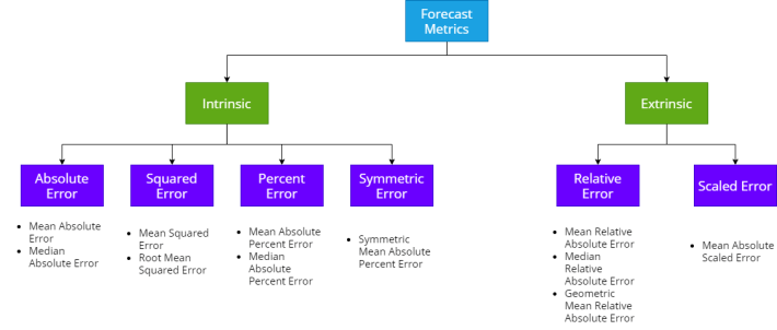
Both Scaled Error and Relative Error are extrinsic error measures. They depend on another reference forecast to evaluate itself, and more often than not, in practice, the reference forecast is a Naïve Forecast or a Seasonal Naïve Forecast. In addition to these errors, we will also look at measures like Percent better, cumulative Forecast Error, Tracking Signal etc.
Relative Error
When we say Relative Error, there are two main ways of calculating it and Shcherbakov et al. calls them Relative Errors and Relative Measures.
Relative Error is when we use the forecast from a reference model as a base to compare the errors and Relative Measures is when we use some forecast measure from a reference base model to calculate the errors.
Relative Error is calculated as below:


Similarly Relative Measures are calculated as below:

where 

Relative Error is based on a reference forecast, although most commonly we use Naïve Forecast, not necessarily all the time. For instance, we can use the Relative measures if we have an existing forecast we are trying to better, or we can use the baseline forecast we define during the development cycle, etc.
One disadvantage we can see right away is that it will be undefined when the reference forecast is equal to ground truth. And this can be the case for either very stable time series or intermittent ones where we can have the same ground truth repeated, which makes the naïve forecast equal to the ground truth.
Scaled Error
Scaler Error was proposed by Hyndman and Koehler in 2006. They proposed to scale the errors based on the in-sample MAE from the naïve forecasting method. So instead of using the ground truth from the previous timestep as the scaling factor, we use the average absolute error across the entire series as the scaling factor.

where 


Here in-sample MAE is chosen because it is always available and more reliable to estimate the scale as opposed to the out of sample ones.
Experiments
In our previous blog, we checked Scale Dependency, Symmetricity, Loss Curves, Over and under Forecasting and Impact of outliers. But this time, we are dealing with relative errors. And therefore plotting loss curves are not easy anymore because there are three inputs, ground truth, forecast, and reference forecast and the value of the measure can vary with each of these. Over and Under Forecasting and Impact of Outliers we can still check.
Loss Curves
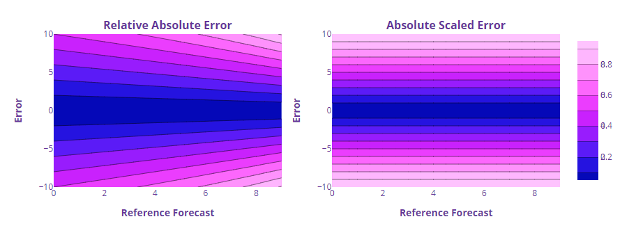
The loss curves are plotted as a contour map to accommodate the three dimensions – Error, Reference Forecast and the measure value.
We can see that the errors are symmetric around the Error axis. If we keep the Reference Forecast constant and vary the error, the measures are symmetric on both sides of the errors. Not surprising since all these errors have their base in absolute error, which we saw was symmetric.
But the interesting thing here is the dependency on the reference forecast. The same error lead to different Relative Absolute Error values depending on the Reference Forecast.

We can see the same asymmetry in the 3D plot of the curve as well. But Scaled Error is different here because it is not directly dependent on the Reference Forecast, but rather on the mean absolute error of the reference forecast. And therefore it has the good symmetry of absolute error and very little dependency on the reference forecast.
Over and Under Forecasting
For the Over and Under Forecasting experiment, we repeated the same setup from last time*, but for these four error measures – Mean Relative Absolute Error(MRAE), Mean Absolute Scaled Error(MASE), Relative Mean Absolute Error(RMAE), and Relative Root Mean Squared Error(RRMSE)
* – With one small change, because we also add a random noise less than 1 to make sure consecutive actuals are not the same. In such cases the Relative Measures are undefined.
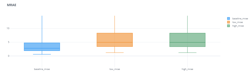

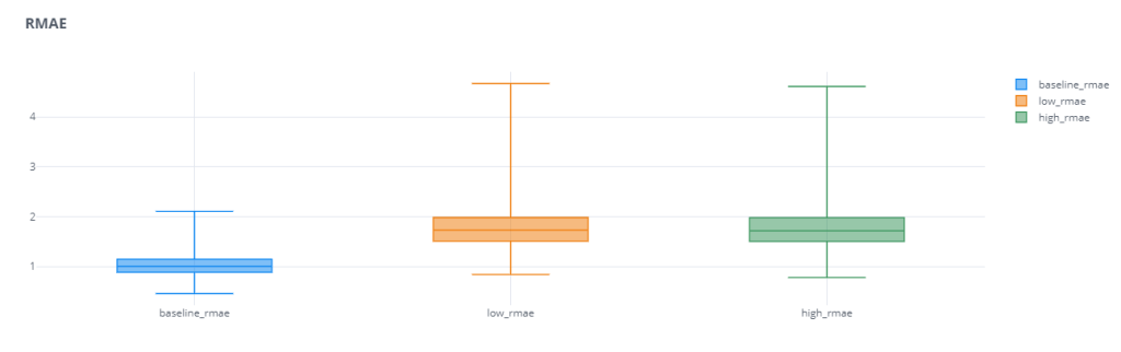
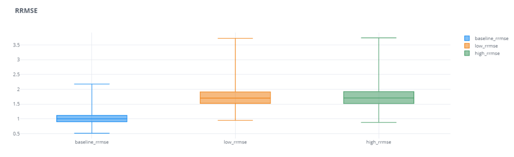

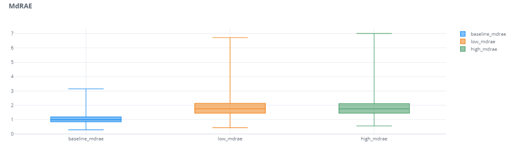
We can see that these scaled and relative errors do not have that problem of favoring over or under forecasting. Both the error bars of low forecast and high forecast are equally bad. Even in cases where the base error was favoring one of these,(for eg. MAPE), the relative error measure(RMAPE) reduces that “favor” and makes the error measure more robust.
One other thing we notice is that the Mean Relative Error has a huge spread(I’ve actually zoomed in to make the plot legible). For eg. The median baseline_rmae is 2.79 and the maximum baseline_mrae is 42k. This large spread shows us that the Mean Absolute Relative Error has low reliability. Depending on different samples, the errors vary wildly. this may be partly because of the way we use the Reference Forecast. If the Ground Truth is too close to Reference Forecast(in this case the Naïve Forecast), the errors are going to be much higher. This disadvantage is partly resolved by using Median Relative Absolute Error(MdRAE)
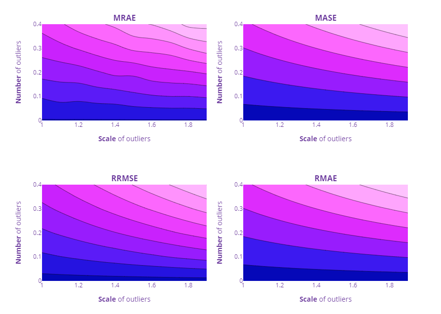
Outlier Impact
For checking the outlier impact also, we repeated the same experiment from previous blog post for MRAE, MASE, RMAE, and RRMSE.
Other Errors
Apart from these standard error measures, there are a few more tailored to tackle a few aspects of the forecast which is not properly covered by the measures we have seen so far.
Percent Better
Out of all the measures we’ve seen so far, only MAPE is what I would call interpretable for non-technical folks. But as we saw, MAPE does not have the best of properties. All the other measures does not intuitively expound how good or bad the forecast is. Percent Better is another attempt at getting that kind of interpretability.
Percent Better(PB) also relies on a reference forecast and measures our forecast by counting the number of instances where our forecast error measure was better than reference forecast error.
For eg.

where I = 0 when MAE>MAE* and 1 when MAE<MAE*, and N is the number of instances.
Similarly, we can extend this to any other error measure. This gives us an intuitive understand of how better are we doing as compared to reference forecast. This is also pretty resistant to outliers because it only counts the instances instead of measuring or quantifying the error.
That is also a key disadvantage. We are only measuring the count of the times we are better. But it doesn’t measure how better or how worse we are doing. If our error is 50% less than reference error or 1% less, the impact of that on the Percent better score is the same.
Normalized RMSE (nRMSE)
Normalized RMSE was proposed to neutralize the scale dependency of RMSE. The general idea is to divide RMSE with a scalar, like the maximum value in all the timeseries, or the difference between the maximum or minimum, or the mean value of all the ground truths etc.
Since dividing by maximum or the difference between maximum and minimum are prone to impact from outliers, popular use of nRMSE is by normalizing with the mean.
nRMSE =RMSE/ mean (y)
Cumulative Forecast Error a.k.a. Forecast Bias
All the errors we’ve seen so far focuses on penalizing errors, no matter positive or negative. We use an absolute or squared term to make sure the errors do not cancel each other out and paint a rosier picture than what it is.
But by doing this, we are also becoming blind to structural problems with the forecast. If we are consistently over forecasting or under forecasting, that is something we should be aware of and take corrective actions. But none of the measures we’ve seen so far looks at this perspective.
This is where Forecast Bias comes in.

Although it looks like the Percent Error formula, the key here is the absence of the absolute term. So without the absolute term, we are cumulating the actuals and forecast and measuring the difference between them as a percentage. This gives an intuitive explanation. If we see a bias of 5%, we can infer that overall, we are under-forecasting by 5%. Depending on whether we use Actuals – forecast or Forecast – Actuals, the interpretation is different, but in spirit the same.
If we are calculating across timeseries, then also we cumulate the actuals and forecast at whatever cut of the data we are measuring and calculate the Forecast Bias.
Summary
Let’s add the error measures we saw now to the summary table we made last time.
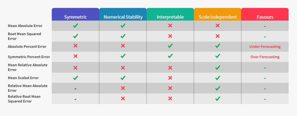
Again we see that there is no one ring to rule them all. There may be different choices depending on the situation and we need to pick and choose for specific purposes.
Thumb-rules and Guide to choosing a Forecast Metric
We have already seen that it is not easy to just pick one forecast metric and use it everywhere. Each of them has its own advantages and disadvantages and our choice should be cognizant of all of those.
That being said, there are thumb-rules you can apply to help you along the process:
- If every timeseries is on the same scale, use MAE, RMSE etc.
- If there are large changes in the timeseries(i.e. in the horizon we are measuring, there is a huge shift is timeseries levels), then something like a Percent Better or Relative Absolute Error can be used.
- When summarizing across timeseries, for metrics like Percent Better or APE, we can use Arithmetic Means(eg. MAPE). For relative errors, it has been empirically proven that Geometric Means have better properties. But at the same time, they are also vulnerable to outliers. A few ways we can control for outliers are:
- Trimming the outliers or discarding them from the aggregate calculation
- Using the Median for aggregation(MdAPE) is another extreme measure in controlling for outliers.
- Winsorizing(replacing the outliers with the cutoff value) is another way to deal with such huge individual cases of errors.
Error Measures for Generalizing About Forecasting Methods: Empirical Comparisons[2]
Armstrong et al. 1992, carried out an extensive study on these forecast metrics using the M competition to sample 5 subsamples totaling a set of 90 annual and 101 quarterly series, and its forecast. Then they went ahead and calculation the error measures on this sample and carried out a study to examine them.
The key dimensions they examined the different measures for were:
Reliability
Reliability talks about whether repeated application of the measure produce similar results. To measure this, they first calculated the error measures for different forecasting methods on all 5 subsamples(aggregate level), and ranked them in order of performance. They carried out this 1 step ahead and 6 steps ahead for Annual and Quarterly series.
So they calculated the Spearman’s rank-order correlation coefficients(pairwise) for each subsample and averaged them. e.g. We took the rankings from subsample 1 and compared them with subsample 2, and then subsample 1 with subsample 3, etc., until we covered all the pairs and then averaged them.
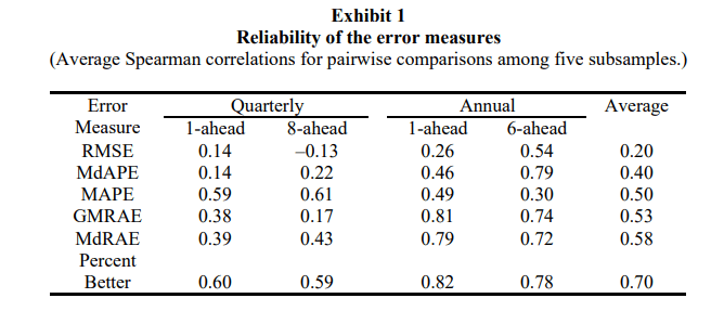
The rankings based on RMSE was the least reliable with very low correlation coefficients. They state that the use of RMSE can overcome this reliability issue only when there is a high number of time series in the mix which might neutralize the effect.
They also found out that Relative Measures like the Percent Better and MdRAE has much higher reliability than their peers. They also tried to calculate the number of samples required to achieve the same statistical significance as Percent Better – 18 series for GMRAE, 19 using MdRAE, 49 using MAPE, 55 using MdAPE, and 170 using RMSE.
Construct Validity
While reliability was measuring the consistency, construct validity asks whether a measure does, in fact, measure what it intents to measure. This shows us the extent to which the various measures assess the “accuracy” of forecasting methods. To compare this they examined the rankings of the forecast methods as before, but this time they compared the rankings between pairs of error measures. For eg., how much agreement is there in ranking based on RMSE vs ranking based on MAPE?
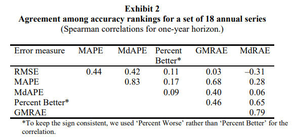
These correlations are influenced by both Construct Validity as well as Reliability. To account for the change in Reliability, the authors derived the same table by using more number of samples and found that as expected the average correlations increased from 0.34 to 0.68 showing that these measures are, in fact, measuring what they are supposed to.

As a final test of validity, they constructed a consensus ranking by averaging the rankings from each of the error measures for the full sample of 90 annual series and 1010 quarterly series and then examined the correlations of each individual error measure ranking with the consensus ranking.
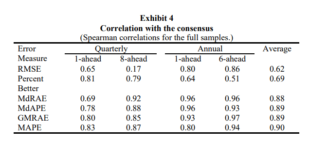
RMSE had the lowest correlation with the consensus. This is probably because of the low reliability. It can also be because of RMSE’s emphasis on higher errors.
Percent Better also shows low correlation(even though it had high reliability). This is probably because Percent better is the only measure which does not measure the magnitude of the error.
Sensitivity
It is desirable to have error measures which are sensitive to effects of changes, especially for parameter calibration or tuning. The measure should indicate the effect on “accuracy” when a change is made in the parameters of the model.
Median error measures are not sensitive and neither is Percent Better. Median aggregation hides the change by focusing on the middle value and will only change slowly. Percent Better is not sensitive because once the series is performing better than the reference, it stops making any more change in the metric. It also does not measure if we improve an extremely bad forecast to a point where it is almost as accurate as a naïve forecast.
Relationship to Decision Making
The paper makes it very clear that none of the measures they evaluated are ideal for decision making. They propose RMSE as a good enough measure and frown upon percent based errors under the argument that actual business impact occurs in dollars and not in percent errors. But I disagree with the point because when we are objectively evaluating a forecast to convey how good or bad it is doing, RMSE just does not make the cut. If I walk up to the top management and say that the financial forecast had an RMSE of 22343 that would fall flat. But instead if I say that the accuracy was 90% everybody is happy.
Both me and the paper agree on one thing, the relative error measures of not that relevant to decision making.
Guidelines for choosing Error Measures
To help with selection of errors, the paper also rates the different measures of the dimensions they identified.
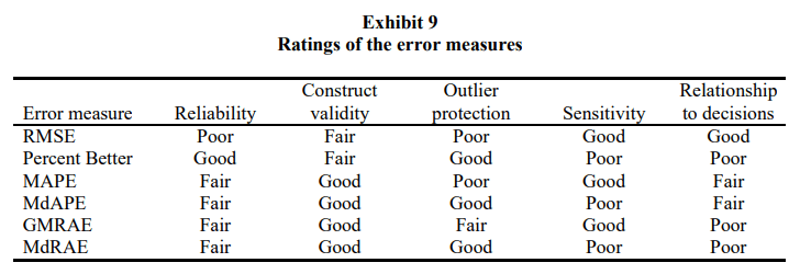
For Parameter Tuning
For calibration of parameter tuning, the paper suggests to use on of the measures which are rated high in sensitivity, – RMSE, MAPE, and GMRAE. And because of the low reliability of RMSE and the favoring low forecast issue of MAPE, they suggest to use GMRAE(Geometric Mean Relative Absolute Error). MASE was proposed way after the release of this paper and hence it does not actor in these analysis. But if you think about it MASE is also sensitive and immune to the problems that we see for RMSE or MAPE and can be a good candidate for calibration.
For Forecast Method Selection
To select between forecast methods, the primary criteria are reliability, construct validity, protection against outliers, and relationship to decision making. Sensitivity is not that important in this context.
The paper, right away, dismissed RMSE because of the low reliability and the lack of protection to outliers. When the number of series is low, they suggest MdRAE, which is as reliable as GMRAE, but offers additional protection from outliers.Given a moderate number of series, reliability becomes less of an issue and in such cases MdAPE would be an appropriate choice because of its closer relationship to decision making.
Conclusion
Over the two blogposts, we’ve seen a lot of forecast measures and understood what are the advantages and disadvantages for each of them. And finally arrived at a few thumb rules to go by when choosing forecast measures. although not conclusive, I hope it gives you a direction when going about these decisions.
But all this discussion was made under the assumption that the time-series that we are forecasting are stable and smooth. But in real-world business cases, there are also a lot of series which are intermittent or sporadic. We see long periods of zero demand before a non-zero demand. under such cases, almost all of the error measures(with an exception of may be MASE) fails. In the next blog post, let’s take a look at a few different measures which are suited to intermittent demand.
Github Link for the Experiments: https://github.com/manujosephv/forecast_metrics
Update – 04-10-2020
Upon further reading, stumbled upon a few criticism of MASE as well, and thought I should mention that as well here.
- There is some criticism on the fact that we use the average MAE of the reference forecast as the scaling error term. Davidenko and Fildes(2013)[3] claims that that introduces a bias towards overrating the accuracy of the reference forecast. In other words, the penalty for bad forecasting becomes larger than the reward for good forecasting.
- Another criticism derives from the fact that mean is not a very stable estimate and can be swayed by a couple of large values.
Another interesting fact that Davidenko and Fildes[3] shows is that MASE is equivalent to the weighted arithmetic mean of relative MAE, where number of available error values is the weight.
Checkout the rest of the articles in the series
- Forecast Error Measures: Understanding them through experiments
- Forecast Error Measures: Scaled, Relative, and other Errors
- Forecast Error Measures: Intermittent Demand
References
- Shcherbakov et al. 2013, A Survey of Forecast Error Measures
- Armstrong et al. 1992, Error Measures for Generalizing About Forecasting Methods: Empirical Comparisons
- Davidenko & Fildes. 2013, Measuring Forecast Accuracy: The Case Of Judgmental Adjustments To Sku-Level Demand Forecasts

2 thoughts on “Forecast Error Measures: Scaled, Relative, and other Errors”