Intermittent Demand Forecasting with Deep Renewal Processes

Let’s face it, anyone who has worked on Time Series Forecasting problems in the retail, logistics, e-commerce etc. would have definitely cursed that long tail which never behaves. The dreaded intermittent time series which makes the job of a forecaster difficult. This nuisance renders most of the standard forecasting techniques impractical, raises questions about the metrics, model selection, model ensembling, you name it. And to make things worse, there may be cases(like in the spare parts industry, where intermittent patterns appear is slow-moving but highly critical or high value items.

Notation

– ith element of the time series

– The index of timeseries

– The index of non-zero demand

– The inter-demand interval, i.e. the gap between two non-zero demand.

– The demand size at non-zero demand point.

Traditional Approach

Traditionally, there is a class of algorithms which take a slightly different path to forecasting the intermittent time series. This set of algorithms considered the intermittent demand in two parts – Demand Size and Inter-demand Interval – and modelled them separately.

Croston

Croston proposed to apply a single exponential smoothing seperately to both M and Q, as below:

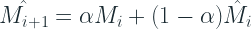
After getting these estimates, final forecast,

And this is a one-step ahead forecast and if we have to extend to multiple timesteps, we are left with a flat forecast with the same value.

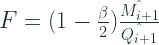
Croston(SBA)

Syntetos and Boylan, 2005, showed that Croston forecasting was biased on intermittent demand and proposed a correction with the from inter demand interval estimation.

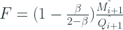
Croston(SBJ)

Shale, Boylan, and Johnston (2006) derived the expected bias when the arrival follow a Poisson process.

Croston Forecasting as Renewal Process

Renewal process is an arrival process in which the interarrival intervals are positive, independent and identically distributed (IID) random variables (rv’s). This formulation generalizes Poison process for arbitrary long times. Usually, in a Poisson process the inter-demand intervals are exponentially distributed. But renewal processes have an i.i.d. inter-demand time that have a finite mean.

Turkmen et al. 2019 casts Croston and its variants into a renewal process mold. The random variables, M and Q, both defined on positive integers fully define the

Deep Renewal Process

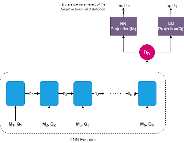
Once Croston forecasting was cast as a renewal process, Turkmen et al. proposed to estimate them by using a separate RNN for each “Demand Size” and “Inter-demand Interval”.

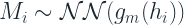
where

This means that we have a single RNN, which takes in as input both M and Q and encodes that information into an encoder(h). And then we put two separate NN layers on top of this hidden layer to estimate the probability distribution of both M and Q. For both M and Q, Negative Binomial distribution is the choice suggested by the paper.

Negative Binomial Distribution

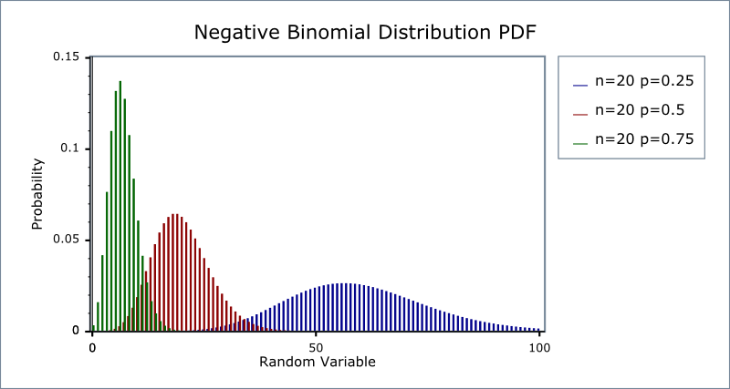
Negative Binomial Distribution is a discrete probability distribution which is commonly used to model count data. For example, the number of units of an SKU sold, number of people who visited a website, or number of service calls a call center receives.

The distribution derives from a sequence of Bernoulli Trials, which says that there are only two outcomes for each experiment. A classic example is a coin toss, which can either be heads or tails. So the probability of success is p and failure is 1-p (in a fair coin toss, this is 0.5 each). So now if we keep on performing this experiment until we have seen r successes, the number of failures we see will have a negative binomial distribution.

The semantic meaning of success and failure need not hold true when we apply this, but what matters is that there are only two types of outcome.

Network Architecture

Our Contribution

The paper just talks about one-step ahead forecasts, which is also what you will find in a lot of Intermittent Demand Forecast literature. But in a real world, we would need longer than that to plan properly. Whether it is Croston, or Deep Renewal Process, how we generate a n-step ahead forecast is the same – a flat forecast of Demand Size(M)/Inter-demand Time(Q).

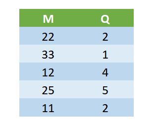
We have introduced a two new method of decoding the output – Exact and Hybrid – in addition to the existing method Flat. Suppose we trained the model with a prediction length of 5.

The raw output from the mode would be:

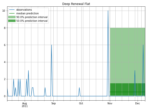
Flat

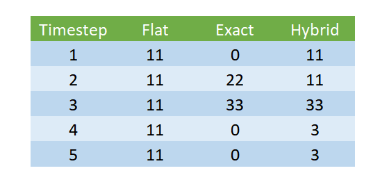
Under flat decoding, we would just pick the first set of outputs (M=22 and Q=2) and generate a one-step ahead forecast and extend the same forecast for all 5 timesteps.

Exact

Exact decoding is more of a more confident version of decoding. Here we predict a demand of demand size M, every Inter demand time of Q and make the rest of the forecast zero.

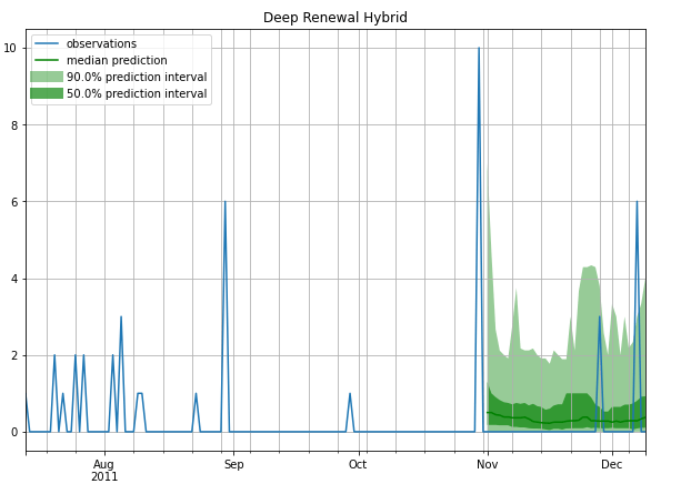
Hybrid

In hybrid decoding, we combine these two to generate a forecast which is also taking into account long-term changes in the model’s expectation. We use the M/Q value for forecast, but we update the M/Q value based on the next steps. For eg, in the example we have, we will forecast 11(which is 22/3) for the first 2 timesteps, and then forecast 33(which is 33/1) for the next timestep, etc.

Implementation

I have implemented the algorithm using GluonTS, which is a framework for Neural Time Series forecasting, built on top of MXNet. AWS Labs is behind the open source project and some of the algorithms like DeepAR are used internally by Amazon to produce forecasts.

Models Implemented

The paper talks about two variants of the model – Discrete Time DRP(Deep Renewal Process) and Continuous Time DRP. In this library, we have only implemented the discrete time DRP, as it is the more popular use case.

How to install?

The package is uploaded on pypi and can be installed using:

pip install deeprenewal

Recommended Python Version: 3.6

Source Code: https://github.com/manujosephv/deeprenewalprocess

If you are working Windows and need to use your GPU(which I recommend), you need to first install MXNet==1.6.0 version which supports GPU MXNet Official Installation Page

And if you are facing difficulties installing the GPU version, you can try(depending on the CUDA version you have)

pip install mxnet-cu101==1.6.0 -f https://dist.mxnet.io/python/all

Relevant Github Issue

Usage

usage: deeprenewal [-h] [--use-cuda USE_CUDA] 
                   [--datasource {retail_dataset}]
                   [--regenerate-datasource REGENERATE_DATASOURCE]
                   [--model-save-dir MODEL_SAVE_DIR]
                   [--point-forecast {median,mean}]
                   [--calculate-spec CALCULATE_SPEC] 
                   [--batch_size BATCH_SIZE]
                   [--learning-rate LEARNING_RATE] 
                   [--max-epochs MAX_EPOCHS]
                   [--number-of-batches-per-epoch NUMBER_OF_BATCHES_PER_EPOCH]
                   [--clip-gradient CLIP_GRADIENT]
                   [--weight-decay WEIGHT_DECAY]
                   [--context-length-multiplier CONTEXT_LENGTH_MULTIPLIER]
                   [--num-layers NUM_LAYERS] 
                   [--num-cells NUM_CELLS]
                   [--cell-type CELL_TYPE] 
                   [--dropout-rate DROPOUT_RATE]
                   [--use-feat-dynamic-real USE_FEAT_DYNAMIC_REAL]
                   [--use-feat-static-cat USE_FEAT_STATIC_CAT]
                   [--use-feat-static-real USE_FEAT_STATIC_REAL]
                   [--scaling SCALING]
                   [--num-parallel-samples NUM_PARALLEL_SAMPLES]
                   [--num-lags NUM_LAGS] 
                   [--forecast-type FORECAST_TYPE]

GluonTS implementation of paper 'Intermittent Demand Forecasting with Deep
Renewal Processes'

optional arguments:
  -h, --help            show this help message and exit
  --use-cuda USE_CUDA
  --datasource {retail_dataset}
  --regenerate-datasource REGENERATE_DATASOURCE
                        Whether to discard locally saved dataset and
                        regenerate from source
  --model-save-dir MODEL_SAVE_DIR
                        Folder to save models
  --point-forecast {median,mean}
                        How to estimate point forecast? Mean or Median
  --calculate-spec CALCULATE_SPEC
                        Whether to calculate SPEC. It is computationally
                        expensive and therefore False by default
  --batch_size BATCH_SIZE
  --learning-rate LEARNING_RATE
  --max-epochs MAX_EPOCHS
  --number-of-batches-per-epoch NUMBER_OF_BATCHES_PER_EPOCH
  --clip-gradient CLIP_GRADIENT
  --weight-decay WEIGHT_DECAY
  --context-length-multiplier CONTEXT_LENGTH_MULTIPLIER
                        If context multipler is 2, context available to hte
                        RNN is 2*prediction length
  --num-layers NUM_LAYERS
  --num-cells NUM_CELLS
  --cell-type CELL_TYPE
  --dropout-rate DROPOUT_RATE
  --use-feat-dynamic-real USE_FEAT_DYNAMIC_REAL
  --use-feat-static-cat USE_FEAT_STATIC_CAT
  --use-feat-static-real USE_FEAT_STATIC_REAL
  --scaling SCALING     Whether to scale targets or not
  --num-parallel-samples NUM_PARALLEL_SAMPLES
  --num-lags NUM_LAGS   Number of lags to be included as feature
  --forecast-type FORECAST_TYPE
                        Defines how the forecast is decoded. For details look
                        at the documentation

There is also a notebook in examples folder which shows how to use the model. Relevant Excerpt is below:

dataset = get_dataset(args.datasource, regenerate=False)
prediction_length = dataset.metadata.prediction_length
freq = dataset.metadata.freq
cardinality = ast.literal_eval(dataset.metadata.feat_static_cat[0].cardinality)
train_ds = dataset.train
test_ds = dataset.test
trainer = Trainer(ctx=mx.context.gpu() if is_gpu&args.use_cuda else mx.context.cpu(), 
                  batch_size=args.batch_size,
                  learning_rate=args.learning_rate,
                  epochs=20,
                  num_batches_per_epoch=args.number_of_batches_per_epoch,
                  clip_gradient=args.clip_gradient,
                  weight_decay=args.weight_decay,
                  hybridize=True) #hybridize false for development

estimator = DeepRenewalEstimator(
    prediction_length=prediction_length,
    context_length=prediction_length*args.context_length_multiplier,
    num_layers=args.num_layers,
    num_cells=args.num_cells,
    cell_type=args.cell_type,
    dropout_rate=args.dropout_rate,
    scaling=True,
    lags_seq=np.arange(1,args.num_lags+1).tolist(),
    freq=freq,
    use_feat_dynamic_real=args.use_feat_dynamic_real,
    use_feat_static_cat=args.use_feat_static_cat,
    use_feat_static_real=args.use_feat_static_real,
    cardinality=cardinality if args.use_feat_static_cat else None,
    trainer=trainer,
)
predictor = estimator.train(train_ds, test_ds)
deep_renewal_flat_forecast_it, ts_it = make_evaluation_predictions(
    dataset=test_ds, predictor=predictor, num_samples=100
)
evaluator = IntermittentEvaluator(quantiles=[0.25,0.5,0.75], median=True, calculate_spec=False, round_integer=True)
#DeepAR
agg_metrics, item_metrics = evaluator(
    ts_it, deep_renewal_flat_forecast_it, num_series=len(test_ds)
)

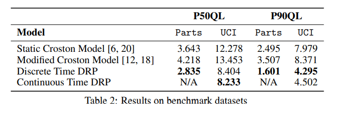
Experiment and Results from the Paper

The paper evaluates the model on two datasets – Parts dataset and UCI Retail Dataset. And for evaluation of the probabilistic forecast, they use Quantile Loss.

The authors used a single hidden layer with 10 hidden units and used the softplus activation to map the LSTM embedding to distribution parameters. They have used a global RNN, i.e. LSTM parameters are shared across all the timeseries. And they evaluated the one-step ahead forecast.

Our Experiments and Contribution

Experiment Setup

We did not recreate the experiment, rather expanded the scope. The dataset chosen was the UCI Retail Dataset, and instead of one step ahead forecast, we took 39 days ahead forecast. This is more in line with a real world application where you need more than one-step ahead forecast to plan. And instead of just comparing with Croston and its variants, we do the comparison also with ARIMA, ETS, NPTS, and Deep AR (which is mentioned as the next steps in the paper).

Dataset

UCI Retail dataset is a transactional data set which contains all the transactions occurring between 01/12/2010 and 09/12/2011 for a UK-based and registered non-store online retail. The company mainly sells unique all-occasion gifts. Many customers of the company are wholesalers.

Columns:

• InvoiceNo: Invoice number. Nominal, a 6-digit integral number uniquely assigned to each transaction. If this code starts with letter ‘c’, it indicates a cancellation.
• StockCode: Product (item) code. Nominal, a 5-digit integral number uniquely assigned to each distinct product.
• Description: Product (item) name. Nominal.
• Quantity: The quantities of each product (item) per transaction. Numeric.
• InvoiceDate: Invice Date and time. Numeric, the day and time when each transaction was generated.
• UnitPrice: Unit price. Numeric, Product price per unit in sterling.
• CustomerID: Customer number. Nominal, a 5-digit integral number uniquely assigned to each customer.
• Country: Country name. Nominal, the name of the country where each customer resides.

Preprocessing:

• Group by at StockCode, Country, InvoiceDate –> Sum of Quantity, and Mean of UnitPrice
• Filled in zeros to make timeseries continuous
• Clip lower value of Quantity to 0(removing negatives)
• Took only Time series which had length greater than 52 days.
• Train Test Split Date: 2011-11-01

Stats:

• # of Timeseries: 3828. After filtering: 3671
• Quantity: Mean = 3.76, Max = 12540, Min = 0, Median = 0
  • Heavily Skewed towards zero

Time Series Segmentation

Using the same segmentation – Intermittent, Lumpy, Smooth and Erratic- we discussed earlier, I’ve divided the dataset into four.

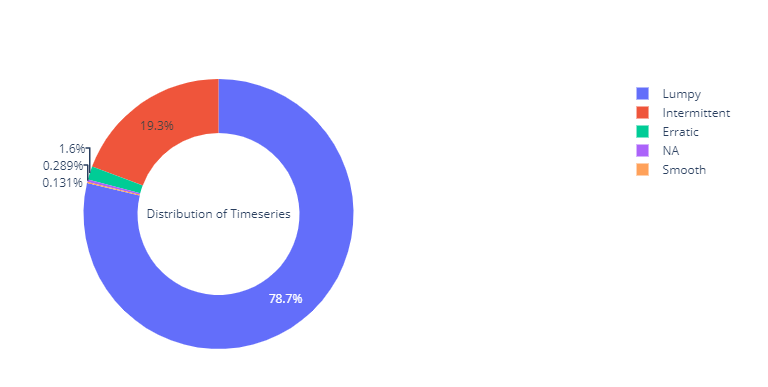
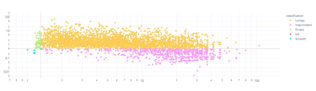
We can see that almost 98% of the timeseries in the dataset are either Intermittent or Lumpy, which is perfect for our use case.

Results

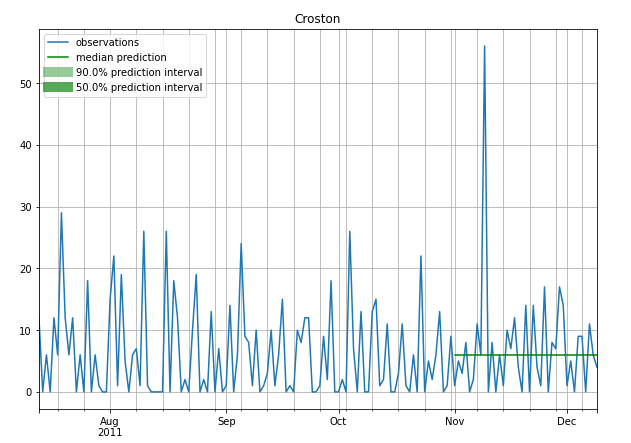
Baseline Comparison

The baseline we have chosen, as the paper, is Croston Forecast. We have also added slight modification to Croston, namely SBA and SBJ. So let’s first do a comparison against these baselines, for both one-step ahead and n-step ahead forecasts. We will also evaluate both point forecast(using MSE, MAPE, and MAAPE) and probabilistic forecast (using Quantile Loss)

We can see that the DRP models have considerably outperformed the baseline methods across both point as well as probabilistic forecasts.

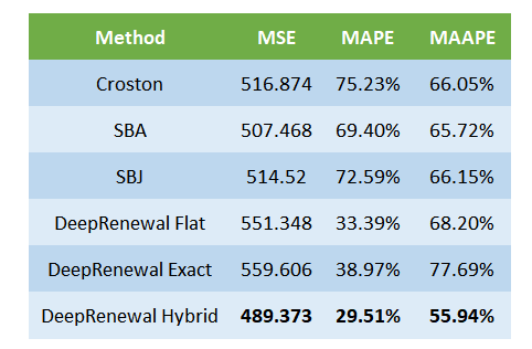
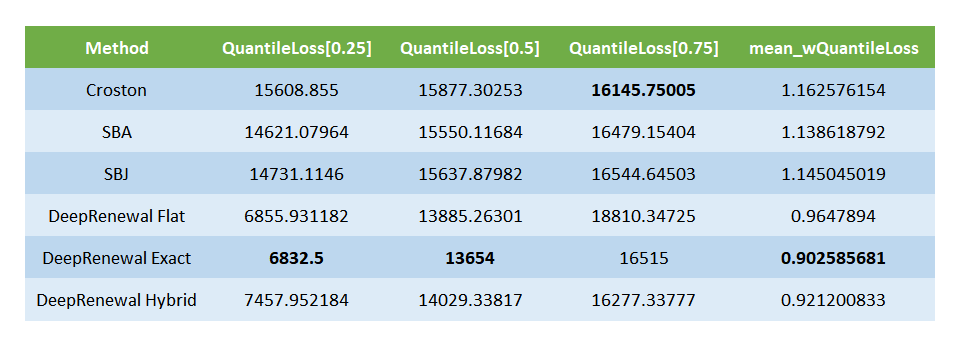
Now let’s take a look at n-step ahead forecasts.

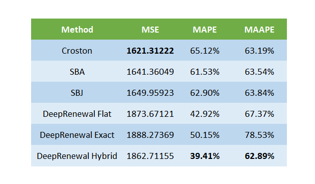
Here, we see a different picture. On the point forecasts, Croston is doing much better on MSE. DRPs are doing well on MAPE, but we know that MAPE favors under forecasting and not very reliable when we look at intermittent demand pattern. So from a point forecast standpoint, I wouldn’t say that DRPs outperformed Croston on long term forecast. What we do notice is that within the DRPs, the Hybrid decoding is working much better than flat decoding, in both MAPE and MSE.

Extended Comparison

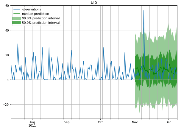
For an extended comparison of the results, let’s also include results from other popular forecasting techniques as well. We have added ETS and ARIMA from the point estimation stable and DeepAR and NPTS from the probabilistic forecast stable.

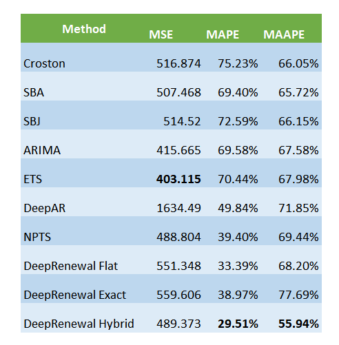
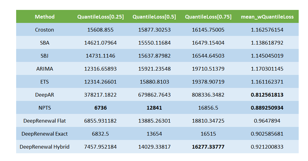
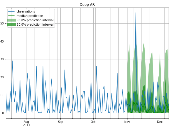
On MSE, ETS takes the top spot, even though on MAPE and MAAPE DRPs retain their position. On the probabilistic forecast side, DeepAR has extraordinarily high Quantile losses, but when we look at a weighted Quantile Loss(weighted by volume) we see it emerging in the top position. This may be because DeepAR forecasting zero(or close to zero) in most of the time and only forecasting good numbers in high volume SKUs. Across all the three Quantile Losses, NPTS seems to be outperforming DRPs by a small margin.

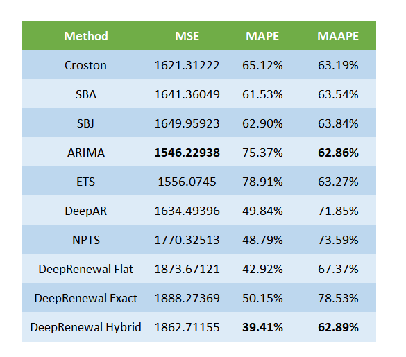
When we look at a long term forecast, we see that ARIMA and ETS is doing considerably better on the point estimates(MSE). And on the Probabilistic side, Deep AR turned it around and managed to become the best probabilistic model.

A few example Forecasts

Intermittent

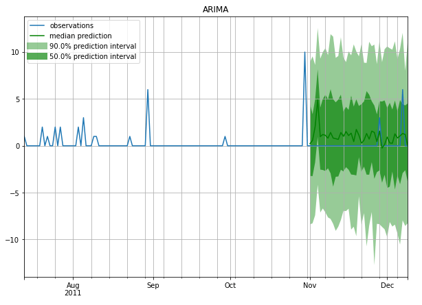
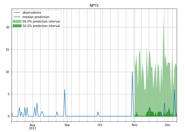
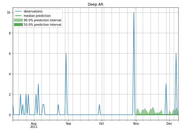
Stable (less Intermittent)

References

Ali Caner Turkmen, Yuyang Wang, Tim Januschowski. “Intermittent Demand Forecasting with Deep Renewal Processes”. arXiv:1911.10416 [cs.LG] (2019)